Text Functions in Excel help you to simplify handling text strings easily. In this article, we’ll learn some of the text functions in Excel.
Also read: Top 10 Logical Functions in Excel – A Quick Reference
Top Text Functions in Excel
Let’s get started with the top text functions present in Excel. We’ll cover the basic use cases along with the function names.
1. CHAR function
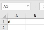
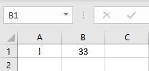
When provided a valid character code, the Excel CHAR function returns a character. The numbers returned by the CHAR function come from ANSI. ANSI stands for American National Standards Institute which is a set of 8-bit characters. These include numbers 0 to 9, lowercase a-z, uppercase A-Z, punctuations, and special characters.
Syntax: CHAR(number), where “number” is an integer between 0-255 and returns a text value. The following example shows the use of CHAR function:
- Select the cell where you want to display the result.
- Type =CHAR(100).
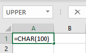
- Press the Enter key to display the result.
2. CLEAN function
All nonprintable characters are removed from the text by the CLEAN function. It also removes line breaks.
Syntax: CLEAN(text), where text is the string that has to be cleaned of line breaks and other non-printable characters. The following example shows the use of CLEAN function:
- Select the cell where you want to display the result.
- Type =CLEAN(, select the cell containing the text and complete the formula with ).
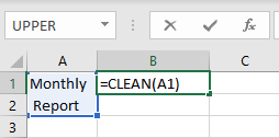
- Press the Enter key to display the result.

3. CODE function
The CODE function returns the first character in a text string as a number code. The character set used by your machine is represented by the ANSI code returned.
Syntax: CODE(text), where text is the character for which the ANSI code is to be returned. The following example shows the use of CODE function:
- Select the cell where you want to display the result.
- Type =CODE(, select the cell containing the text and complete the formula with ).
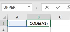
- Press the Enter key to display the result.
4. CONCAT function
The CONCAT function joins text from various ranges and/or strings into a single string. CONCAT function that replaces CONCATENATE in Excel 2016 and above. The CONCATENATE function, on the other hand, will remain accessible for compatibility with older Excel versions.
Syntax: CONCAT(text1, [text2],…), where text1, text2, text3… are the string items to be joined. The following example shows the use of the CONCAT function:
- Select the cell where you want to display the result.
- Type =CONCAT(“Excel”,” “,”2019).

- Press the Enter key to display the result.

5. DOLLAR function
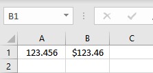
The DOLLAR function in Microsoft Excel transforms a number to text in $ currency format.
Syntax: DOLLAR(number, [decimals]), where number is a reference to a cell containing a number, or a formula that evaluates to a number and decimals is the number of digits to the right of the decimal. The following example shows the use of DOLLAR function:
- Select the cell where you want to display the result.
- Type =DOLLAR(A1,2), where cell A1 contains the number.
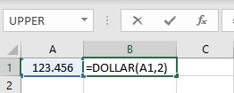
- Press the Enter key to display the result.
6. EXACT function
The EXACT function analyses two text strings and returns TRUE if they are identical, otherwise FALSE. The EXACT function is case-sensitive but overlooks formatting variations.
Syntax: EXACT(text1,text2), where text1 is the first string and text2 is the second string to be compared. The following example shows the use of the EXACT function:
- Select the cell where you want to display the result.
- Type =EXACT(A1,B1), where cells A1 and B1 contain the strings to be compared.

- Press the Enter key to display the result.

7. LEN function
the LEN function returns the number of characters in a string including white spaces in between.
Syntax: LEN(text), where text is the string whose length you wish to find or the cell reference of the cell contains the string. The following example shows the use of LEN function:
- Select the cell where you want to display the result.
- Type =LEN(, select the cell containing the text and complete the formula with ).
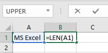
- Press the Enter key to display the result.
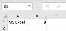
The text string “MS Excel” contains 7 characters and 1 blank space.
8. FIND function
The FIND function in Excel returns the starting position of one text string within another text string.
Syntax: FIND(find_text, within_text, [start_num]), where find_text is the text you wish to find, within_text is the text within which you want to find for a particular string. start_num is an optional parameter that specifies the position from which to start the search. The following example shows the use of the FIND function:
- Select the cell where you want to display the result.
- Type =FIND(“x”,A1), where cell A1 contains the string to be searched for character “x”.
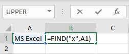
- Press the Enter key to display the result.
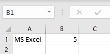
The character “x” is located at the 5th index position in the string “MS Excel”.
9. REPLACE function
The REPLACE function replaces a portion of a text string with a different text string based on the number of characters you specify.
Syntax: REPLACE(old_text, start_num, num_chars, new_text), where:
- old_text is the text from which you wish to replace a portion
- start_num is the position in old_text of the character you want to replace with new_text
- num_chars is the number of characters you want REPLACE to replace in old_text with new_text
- new_text is the text that will be used to replace the characters in old_text.
The following example shows the use of REPLACE function:
- Select the cell where you want to display the result.
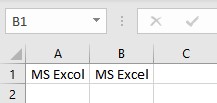
- Type =REPLACE(A1,7,1,”e”), where cell A1 contains the old_text, 7 is the index position of the character to be replaced, 1 is the length of the new_text, and “e” is the character to be placed.

- Press the Enter key to display the result.
Conclusion
In this article, we learned about some of the most commonly used text functions in Excel.
