In this article, we’ll learn how to superscript and subscript in Excel. These are common in technical expressions and will certainly come in handy when dealing with data. Superscripts and subscripts are easy to apply in Excel only if you know how to approach the settings and shortcuts properly.
Also read: [Step-by-Step] How to Round Numbers in Excel?
Format Text as Superscript in Excel
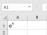
A superscript is a smaller character than the rest of the text which is placed slightly above the baseline e.g. ex, where x is the superscript. Follow these steps to format text as superscript:
- Select the characters in a cell which you want to format as superscripts.
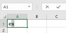
- Click on the Font Settings dialog box launcher present at the bottom right corner in the Font group on the Home tab.

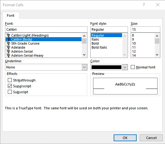
- In the Format Cells dialog box, check the Superscript box under the Effects section and click OK.
This is the result of superscript formatting:
Format Text as Subscript in Excel
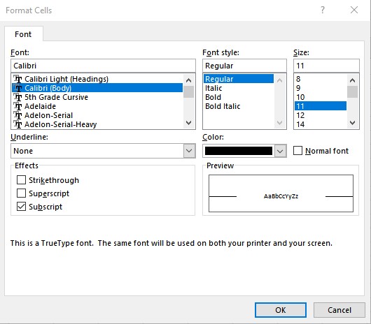
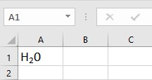
A subscript in excel is a smaller character than the rest of the text which is placed slightly below the baseline e.g. H2O, where 2 is the subscript. Follow these steps to format text as subscript:
- Select the characters in a cell which you want to format as a subscript.
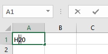
- Click the Font Settings dialog box launcher present at the bottom right corner in the Font group on the Home tab.

- In the Format Cells dialog box, check the Subscript box under the Effects section and click OK.
This is the result of subscript formatting:
Adding Superscript and Subscript Buttons to the Ribbon
Subscript and superscript buttons can be added to the Excel ribbon for quick and easy access just like it is available in Word. Follow these steps to add custom buttons:
- Right-click anywhere on the Excel ribbon. From the options that appear click on Customize the Ribbon… option.

- Excel Options dialog box appears.
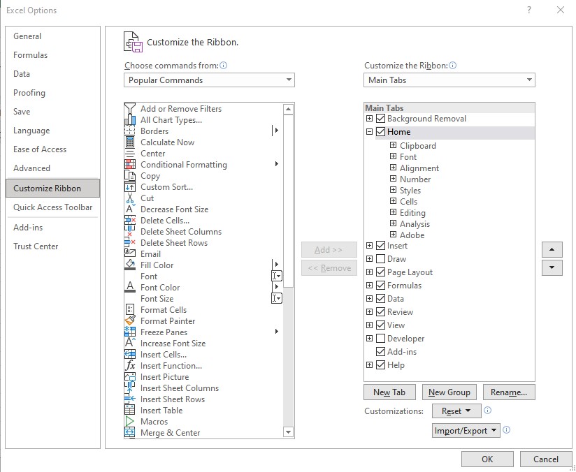
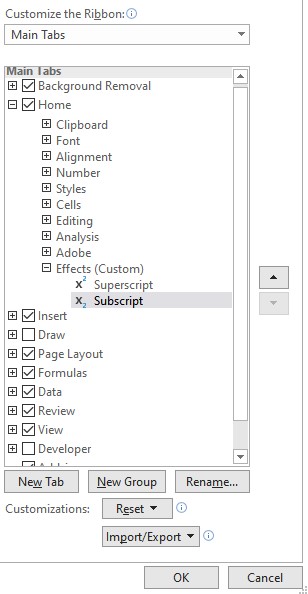
- On the right side of the Excel Options dialog box, under Customize the Ribbon, select the tab where you want to feature the custom buttons. In this example, we have selected the Home tab.
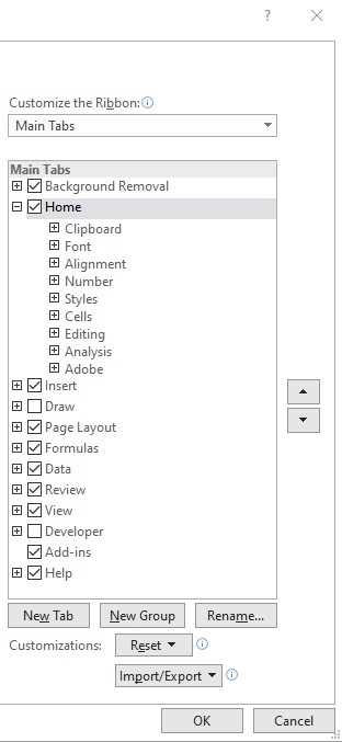
- Click on the New Group button to add a custom group on the Home tab.
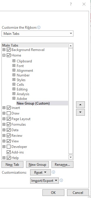
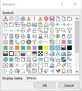
- Click Rename to open the Rename dialog box.

- Name the custom group name by typing in the Display name: text box and click OK. Here, we have named the custom group as Effects.
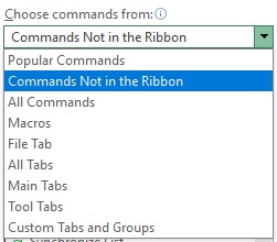
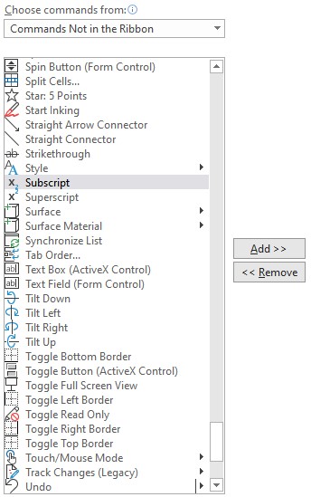
- From the left side drop-down list, under Choose commands from:, select Commands Not in the Ribbon option.
- From the list of commands that appears, select Superscript and then click on Add button.
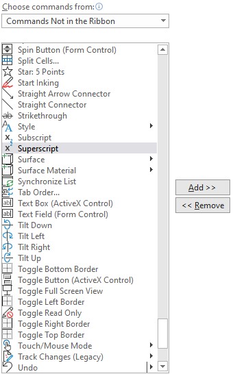
- From the list of commands that appears, select Subscript and then click on Add button.
- You can see that the superscript and subscript buttons are added in the Effects group on the Home tab. Then, click on OK.
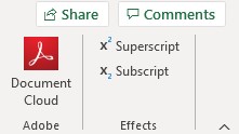
You can now see the buttons in the Effects group on the Home tab for easy access.
Note: This feature is only available with Excel 2016 or above and Office 365 subscriptions.
Also read: [Ultimate Guide] How to Create a Form in Excel?
Adding subscript and superscript buttons to Quick Access Toolbar
Follow these steps to add subscript and superscript buttons to the Quick Access Toolbar (QAT) present at the top of the Excel window:
- In the upper left corner of the Excel window, click on the down arrow next to the Quick Access Toolbar.

- From the Customize Quick Access Toolbar, select the More Commands… option.
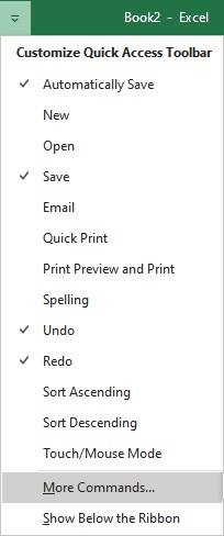
- From the left side drop-down list, under Choose commands from:, select Commands Not in the Ribbon option.
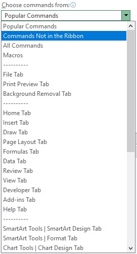
- From the list of commands that appears, select Superscript and then click on Add button.

- From the list of commands that appears, select Subscript and then click on Add button.

- You can see that the superscript and subscript buttons are added in the Quick Access Toolbar. Then, click on OK.
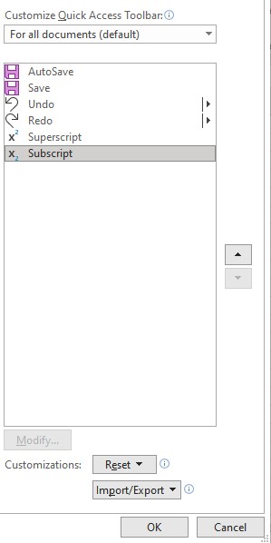
You can now see the buttons in Quick Access Toolbar for easy access.
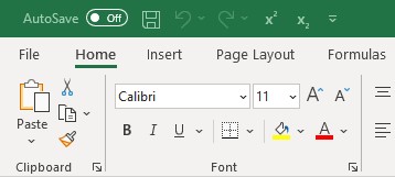
Note: This feature is only available with Excel 2016 or above and Office 365 subscriptions.
Super Easy Way – Simply Copy and Paste from Google
As in Microsoft Excel, it is relatively difficult to format characters, symbols, or numbers as superscripts or subscripts. The easiest and simple way is to search for that character, symbol, or number as superscript or subscript in Google and then simply copy-paste them in an Excel worksheet as per the requirement.
Simply type that character, symbol, or number and add “subscript” or “superscript” in the search bar of Google, and voila, you can now just simply copy-paste without having to do any hard work.
Remove subscript and superscript formatting
- Select the range of cells from where you want to remove the formatting.
- Right-click and select the Format Cells… option.
- In the Format Cells… dialog box, click on the Font tab.
- Clear the Superscript or Subscript checkbox to remove the formatting.
Conclusion
In this tutorial, we learned how to format mathematical expressions and chemical formulas in an appropriate form using superscripts and subscripts respectively. As Excel, doesn’t have by default shortcut buttons for subscript and superscript, we can manually add them by methods discussed in this tutorial.
