You can add a group of numbers listed in a spreadsheet without breaking a sweat, but what if there comes a stipulation amidst this task? How about a list of positive & negative numbers and the task in hand is, to sum up only those which are positive! Now how do ya’ like it?
Also read: How to use AutoSum in Excel? [Step-By-Step]
Yep, that’s life! It always gets you off guard & it ain’t about how hard you hit, but how hard you get hit & get back up on your feet! So in this article, we would be looking into what MS Excel has got to offer to save our feet in this treacherous feat.
Here is the dataset that we would be using for demonstration throughout this article.
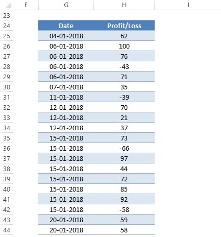
One can observe a sporadic distribution of positive & negative numbers recorded as profits & losses respectively across various dates. We shall now attempt to add only the profits (i.e) only the positive numbers from the above table.
Summing up the Positives:
To make it happen we would summon an in-built feature of MS Excel – the SUMIF formula!
Following is its syntax & by the way, syntax expresses the basic constructs of a formula which makes it work in the first place.
=SUMIF( range, criteria, sum range )
where,
- range – denotes the list of data which would be tested for a specific condition
- criteria – indicates the test condition
- sum range – the range of cells whose data is to be summed up
Let us apply this same logic to the task in hand too & construct a SUMIF to serve the purpose. As with all formulae, SUMIF also starts with an equals sign (=) which should now be obvious after having a look at the syntax given above.
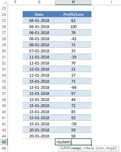
Once the equals is typed into the cell at the very bottom of the Profit/Loss column include an open parenthesis within which the elements of the formula would be keyed in. The first element to take its place would be the range upon which we are going to test whether the numbers present are positive or not.
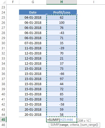
All the cells with numerical data under the Profit/Loss column are selected as shown in the above image. This shall next be followed by placing a comma (,) right next to the range without any spaces & the formula shall prompt you to enter the criteria as indicated in the image below.
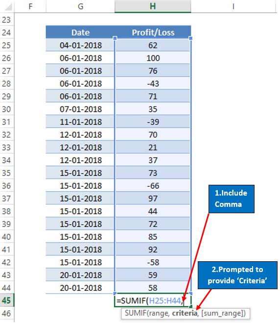
Guess what the criteria might be? Running out of ideas?
Let us have a quick recap on why this formula is being constructed. Yep, for summing up only the positive numbers. So, the criteria should also reflect the same.
There is this elementary concept called ‘number line’ which tells us that anything that falls in the number line behind zero shall belong to the negative group of numbers & those which fall after zero belong to the positive group of numbers.
Simplifying the above statement further would get us,
- numbers < 0 – Negative
- numbers > 0 – Positive
There it is! The criteria for our formula “>0”. We shall now place the criteria within the formula in the exact same way it is expressed – within the double quotes. The final part of the SUMIF formula is more obvious, the same range which we select for the first element of this formula. Once done include a closing parenthesis at the end.
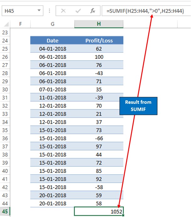
Now it’s time that we hit ENTER & reveal the result.
Conclusion:
Now that we have reached the end of this article, here’s another that details using auto sum in MS Excel. There are numerous other articles too in QuickExcel that can come in handy for those who are in looking to level up their skills in MS Excel. Cheers!
