When it comes to basic arithmetical operations, these two go as far back as elementary education. One amongst them is addition, whilst the other is subtraction. We are going to look into the latter in this article and explore the ways of carrying it out using MS Excel.
Also read: How to Add in Excel? [Easy Guide]
Following is the sample table which we would be using in this article.

Now, let’s calculate the profit made by selling each of the above-listed products. The method which we would adopt for finding the profit, in this case, is called The Operand Method.
Using The Minus Operator in Excel
As always, any formula in MS Excel gets started with an equal to sign “=”. So, we get things started by typing the equal to sign “=” as shown below.

The logic to be applied here is to remove the Buying Price from the Selling Price for each item such that we would be left with the profit gained by selling each product. So, here we would be selecting the cell L3 first.

Once done, it’s time to introduce the operand for subtraction. The operand is the symbol that we use in MS Excel to carry out any specific operation. In this case, we would be using the minus symbol (-) between the two variables to carry out the operation.

Click on the Buying Price of the Chips now, which would be cell K3 to complete the formula.

Hit ENTER and the profit resulted from subtracting the Buying Price from the Selling Price of the Chips would appear in no time.

Similarly, the profit gained by selling the other products can also be calculated by this method. But, there is good stuff! We need not repeat all the steps that we did earlier again.
God bless Copy & Paste!
This time, we are going to copy the formula by copying the cell M3 & pasting it over the cells M4 and M5. Press CTRL + C to copy the contents and then select the cells in which they are to be pasted. Once done, hit CTRL + V to paste the contents into the selected cells.

When one sees a result similar to the one displayed in the above image, it means that things are done & we have accomplished the task of subtracting two numbers using MS Excel.
The copying & pasting can also be done using an old school mouse right-click, rather than a keyboard shortcut for those who are fond of using the mouse.
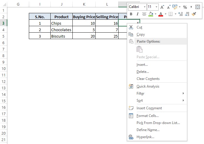
Right-click the selected cell whose formula is to be copied and one can immediately see the following list of options appearing.

Click on Copy in the list of options & then select the cells into which the copied formula is to be pasted.

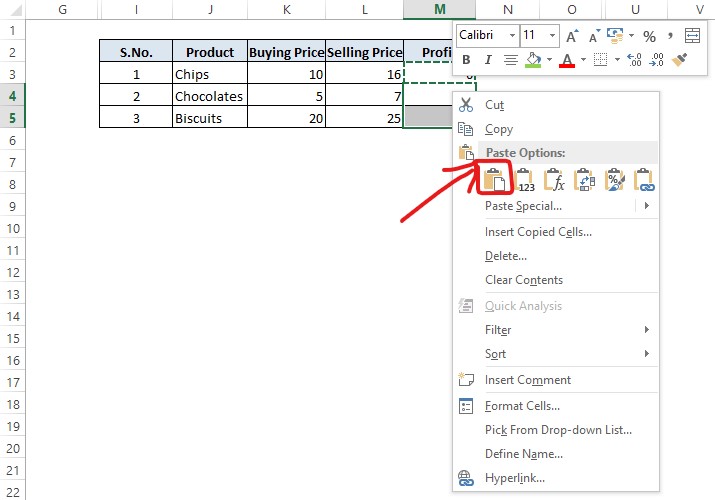
After selecting the cells, right-click using the mouse anywhere within the selected region & again a list of options to choose from would appear. This time click the Paste icon as shown in the below image.

The formula would be successfully copied to the destination and the results would be displayed in a jiffy!
So now we have come across not only how to construct a formula to subtract using an operand, but also to copy and paste it to the other cells as well.
Conclusion
Hope the article was informative. Do have a look at this article, to know how to add numbers using MS Excel. QuickExcel also has numerous other articles, which could help you in many ways to use MS Excel. Ciao!
