In this tutorial, we’ll learn how to pull geographical data in Excel. Getting geographical data of any country, region, or city using the traditional method of manual ‘Google’ or ‘Bing’ searching or ‘Wikipedia’ is time-consuming as well.
Also, directing the way to possible errors while copy-pasting of these data points. Multiply these efforts when pulling geographical data of multiple locations.
Excel helps us fetch and display the geographical data with an add-in.
In this tutorial, we will guide you step-by-step, so you can easily fetch Geographical Data from any region around the globe.
Also read: Genuine Ways to Recover Unsaved and Corrupted Excel Files
What Geographical Data can be fetched in Excel?
Excel’s built-in ‘Stock Market’ tool supports many data parameters which can be fetched directly. These parameters are listed below:
| 01. Abbreviation | 02. Admin Division 1 (State/province/other) | 03. Agricultural land (%) |
| 04. Area | 05. Armed forces size | 06. Birth rate |
| 07. Calling code. | 08. Capital/Major City | 09. Carbon dioxide emissions |
| 10. County/Region | 11. CPI | 12. CPI Change (%) |
| 13. Currency code | 14. Electric power consumption | 15. Fertility rate |
| 16. Forested area (%) | 17. Fossil fuel energy consumption | 18. Gasoline price |
| 19. GDP | 20. Gross tertiary education enrollment (%) | 21. Image |
| 22. Infant mortality | 23. Largest city | 24. Latitude |
| 25. Leader(s) | 26. Life expectancy | 27. Longitude |
| 28.Market cap of listed companies | 29. Maternal mortality ratio | 30. Minimum wage |
| 31. Name | 32. National anthem | 33. Official Language |
| 34. Official name | 35. Out of pocket health expenditure (%) | 36. Physicians per thousand |
| 37. Population | 38. Population: Income share fourth 20% | 39. Population: Income share highest 10% |
| 40. Gross primary education enrollment (%) | 41. Population: Income share highest 20% | 42. Population: Income share lowest 10% |
| 43. Population: Income share lowest 20% | 44. Population: Income share second 20% | 45. Population: Income share third 20% |
| 46. Population: Labor force participation (%) | 47. Subdivisions | 48. Tax revenue (%) |
| 49. Time zone(s) | 50. Total tax rate | 51. Unemployment rate |
| 52. Urban population | — | — |
The important point to note over here is, that all these Data parameters are only available for the County level geographical data points and not all are applicable on Region or City level.
For instance, City – Geographical data parameters that are supported are Abbreviation, Area, Capital/Major City, Country/region, Image, Largest city, Leader(s), Name, Population, and Time zone(s).
Steps to Pull Geographical Data in Excel
Let’s get started with using the ‘Geography’ tool in Excel to get the Geographical details of any region.
Step 1. Organize the Data – Country, Region or City name
Type a country, state, province, territory, or city name into each cell, for which you want to fetch the Geographical details.
You may also enter data points in a table for multiple geographical locations.

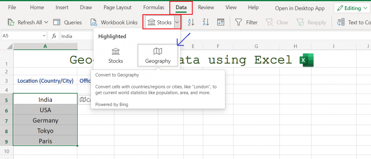
In our example above, we are finding Geography Data of these countries and cities:
India, USA, Germany, Tokyo, Paris – we have purposely used both countries and cities to illustrate a better example in this tutorial. You may also notice that we are using a short form abbreviation for the United States of America. All this is done to show the capabilities of the Excel built-in Geography tool.
Step 2. Select Location and convert to Geography
- Select the cells with Location name or names to get data.
- Navigate to ‘Data‘ in the above tools tab (Home tab)

- Click on ‘Geography‘ to convert the input location names to Geography. [as shown below, the Excel will automatically convert and map the data to the most accurate understanding of Excel tool]

If converted successfully, you will see a map-like symbol just before the entered name/s in the same cell.
Unable to convert to Geography in Excel
In case, after following the above step, your input name wasn’t converted to Geography, a question mark sign appears instead of a map sign.
It’s likely because Excel is having issues matching your text with data. Possible solutions to this are:
Correct any spelling mistakes if you have made or try to be more specific. Or, click on the info symbol to reveal a side pop-up where you will be presented with the option to select the closest matching search results for which Excel will do its best to find matching information
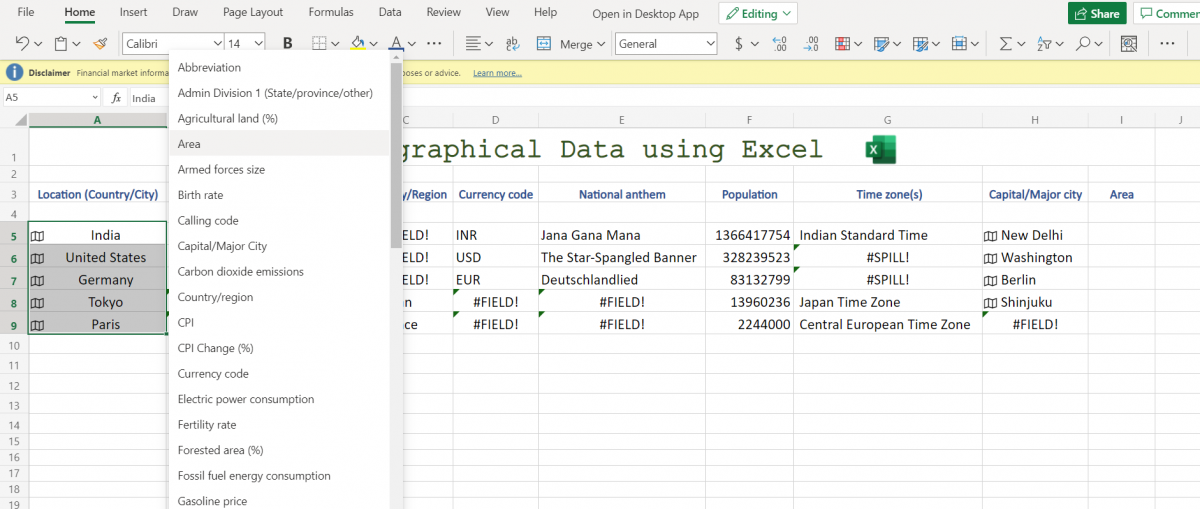
Step 3. Select the Geography parameter for Data
- Excel supports various Geography data parameters to select from, which are shown in the above table here.
- To select particular data parameters, select all the inputted names (converted to geography) and on hovering over them you will be presented with a symbol of data (of somewhat like a book)
- Click on the icon and select the parameter you want to fetch data of.
To see all of the fields available, click the geography icon or select the cell and press ‘Ctrl+Shift+F5‘.
Pro Tip: Set ‘Column Width’ to ‘AutoFit Column Width’ as this sets column width as per the data value inside that particular column, hence, benefiting us in full data value visibility returned by a function.

Final Sheet with all the required data. [You may choose any number of data parameters as per your requirement]:

Note:
#FIELD! – means that Excel was unable to fetch the geographical data of that particular data set. In this case, you may notice the reason for it, it’s pretty obvious how can cities have an Official Name (Tokyo, Paris) hence, #FIELD!. Again, how can a country have a country/region data set hence again unavailability of data?
#SPILL! – simply means out of bound. Which is resultant when a large number of values are returned. Here, in our example it’s evident in Time zone(s) for the United States and Germany because both these countries have multiple time zones and all can’t be fit in a single cell.
##### – the data value is relatively large (long) and doesn’t fit in that cell size. Increase column width or set it to auto to render this error in the data set.
Conclusion
That’s It! You can get Geographical data in various parameters easily by following the above step-by-step procedure now, in your Excel sheets.
We hope you learned and enjoyed this lesson and we’ll be back soon with another awesome Excel tutorial!
