How to Print Gridlines in Excel?

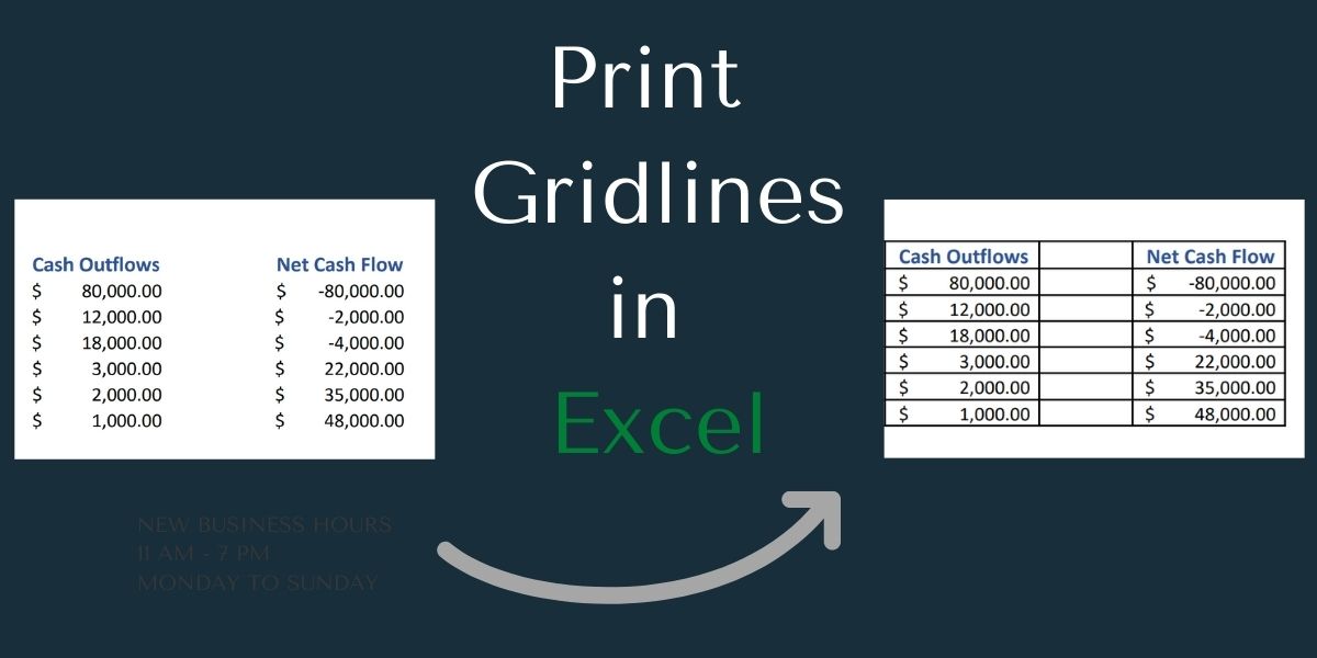
Excel spreadsheets are made up of rows and columns and ‘cell’ is the block where these rows and columns meet. These rows and columns make up for a Grid which collectively is termed as gridlines as they are in line formatting.

By default, printing of Excel worksheet doesn’t include the gridlines of the worksheet rather only blank page is printed (with no lines) with the data values inputted.

Recommended Read: How to Print an Excel Spreadsheet

But, there are times and use case scenarios where you may require to print the gridlines of your Excel Spreadsheet for better and easier readability of data and clear distinction between cell values.

Steps to Print Gridlines in Excel

Follow this below step-by-step tutorial to print gridlines in an Excel spreadsheet or make the gridlines appear in your printed worksheets.

Software Version

Let’s start with the offline version of Excel that you install on your PC. If you’re using Office 365 online, scroll further for the steps for online excel.

Step 1: Select the Print area in spreadsheet

Select the worksheet you want to print.
Now drag and select all the cell values which you want to print to highlight them
Also, you may leave it not selected if you wish to print the whole view-port of the worksheet.

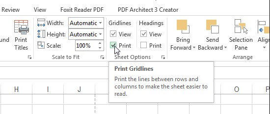
Step 2: Enable Gridlines

From the top options row, click on the Page Layouts tab.
Under Gridlines in the sheet option group, below to the View option
Click to check mark the Print option, which stands for Print Gridlines.

Select Print to print with gridlines in Excel — Select Print to print with gridlines

Step 3: Print the sheet with Gridlines

Click and open the File menu, and then
Click the Print button to print your selected worksheet with gridlines.
Alternatively, you may also use the shortcut Ctrl+P to print the Excel worksheet

For Web Version

We need to mimic gridlines in the Web Version of Excel by using borders as the Web version doesn’t come with the support of gridlines show option.

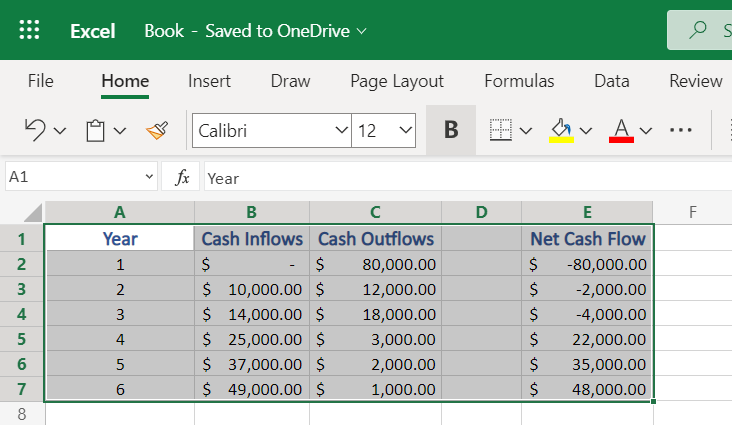
Step 1: Select the cells

Drag and select all the cells that you wish to include in your printing and want to apply a border around.

Selecting cells to apply Borders in Excel — Selecting cells to apply Borders

Step 2: Apply Borders to the selected cells

To mimic gridlines, we now need to apply borders to our selected cells in our Excel spreadsheet.
Go to Home in the above options tab.
Now go to Borders (icon) under font styling group, click on it to reveal a drop-down menu
From the menu select All Borders only to apply accurate replica of gridlines.

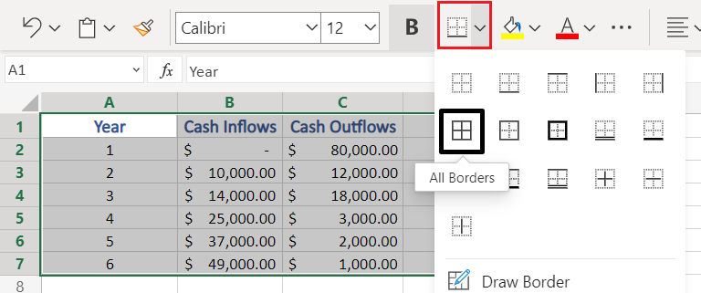
Applying Borders to the cells in Excel — Applying Borders to the cells

Selecting this, would apply the Border styling to all the selected cells and now you are good to go with your printing.

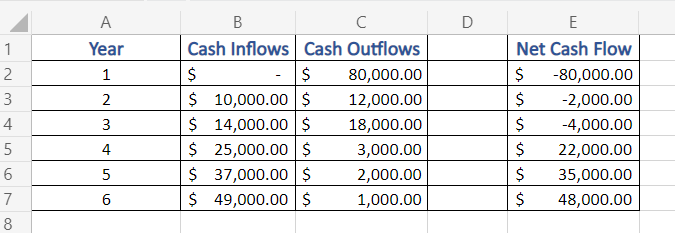
Borders applied to selected cells in Excel — Borders applied to selected cells

Step 3: Print the Sheet

Now as we have added the borders (grids of rows and columns) to our selected cells, to print,
Go to File in the Home row
Click on Print, this will open a print preview window with some print options customization in the right hand option menu.
But, the thing for us to notice here from the print preview is, that our spreadsheet is now printable with Gridlines.

Final Print Preview With Gridlines in Web Version in Excel — Final Print Preview With Gridlines in Web version

Conclusion

We hope you learned how to print out gridlines in Excel with this tutorial. We’re coming up with new and advanced tutorials on a regular basis and will continue to do so! Stay tuned if you’re interested in learning more 🙂