The payback period as by its name is the number of years (or amount of time) it takes to recover the initial capital back from an investment. From investing point of view, every investor has a defined target or tolerance level as for how long they are willing to wait for a return from the investment they make. It is calculated using the after-tax cash flows only.
It is one of the popular accounting terms or methods which are used to calculate the investment strategies and returns of an investment namely, Internal Rate of Return (IRR), Net Present Value (NPV), Payback Period, etc., as this is all investors need to make a decision as these capital budgeting factors help analyze the internal and working prospects of an investment.
For example, if a payback period is stated as 5 years, it means it will take 5 years for the investment to pay the entire initial investment back.
Advantage:
Easy to calculate and also simple to evaluate and analyze.
Disadvantage:
The accounting method is not completely dependable as it does not consider some critical capital budgeting components, as market valuation, inflation (value of money), external factors, and lastly demand and supply.
Steps to Calculate Payback Period in Excel
Without any further ado, let’s get started with calculating the payback period in Excel.
Step 1. Build the dataset
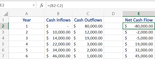
- Enter financial data in your Excel worksheet.
- If your data contains both Cash Inflows and Cash Outflows, calculate “Net Cash flow” or “Cumulative Cash flow” by applying the formula:
- =Cash Inflows – Cash Outflows, as shown below in our example [B2-C2]
Step 2. Break-even Point – Years with Negative Cash Flow
Now, as you input the data values and calculate the Net Cash Flow, let’s start with the main steps:
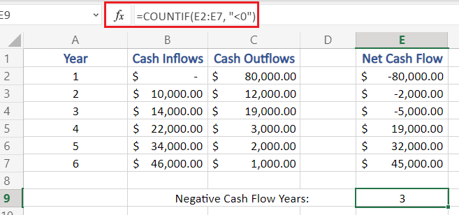
- We need to calculate Number of Years in which the Cash Flow is Negative (-)
- To perform this, we use COUNTIF function as:
=COUNTIF({all values in cash flow column}, “{check}”)
- Here, in our example we apply this as, by selecting all the data values in the Net Cash Flow column and then checking for those which are less than 0(<0) which means, negative
=COUNTIF(E2:E7, “<0”)
What is the Break-even point and why do we calculate it?
When the cumulative cash flows exceed the initial investment, it is termed as the break-even point of the project (The break-even point is the point of no profit and no loss). The time taken to reach (years) the break-even point is the Payback Period. But this Payback period is approximate and not exact. To calculate the exact payback period we apply the next steps.
Step 3. Last Negative Cash Flow
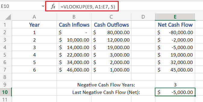
- Now, we calculate the negative cash flow which is the most recent, in other words the last or latest negative cash flow.
- Even though we may look at the Net Cash Flow column and find it, but here in our example we will do the same using function in Excel
- To find the last negative cash flow we use the VLOOKUP function, which takes three arguments as for our usage.
=VLOOKUP(Lookup value, Table array(complete), Column index)
Lookup Value is the value which from whose count we intend to search for (here, negative cash flow years – in cell E9)
Table array is the selection of the whole table values (here, A1:E7)
Column Index is the index of the column where we need to find our value (here, 5th column)
=VLOOKUP(E9, A1:E7, 5)
Step 4. Cash Flow in the Next Year
- Now we calculate the estimated Cash flow for the next year.
- As the formula used in previous step, we need to make some modification to it
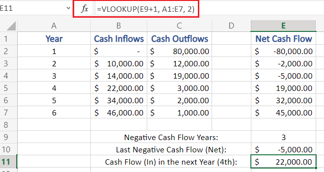
=VLOOKUP(Lookup value + 1, Table array(complete), Column index)
Lookup value is incremented by 1 as we need to get the cash flow of next year
Also, now we need to search for in the column of Cash Inflows, (2nd column)
VLOOKUP(E9+1, A1:E7, 2)
Step 5. Fraction Year Value (month)
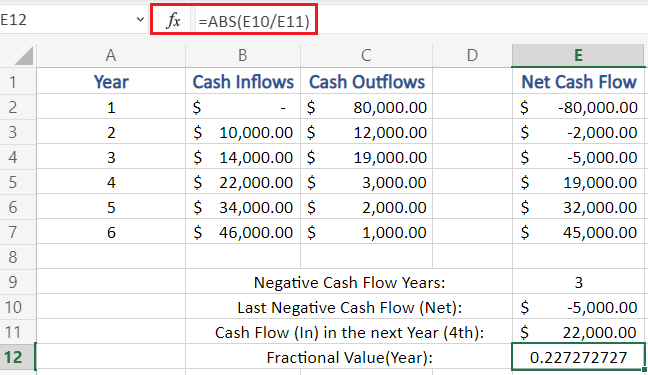
- Calculate the fractional value of year
- This fractional value is calculated as (Last Negative Cash Flow / Cash Flow in Next Year)
- This fractional value is used to know the exact month number for payback period.
- As fractional value represent month of an year, it cannot be negative, hence, we use the absolute function – ABS
=ABS(last negative cash flow/cash flow in next year)
In our example, fractional value is calculated as:
=ABS(E10/E11)
Step 6. Total Payback Period
- The Final Step, as now we have calculated both negative cash flow years (years to reach break-even point) and fraction value (exact years/months of payback period)
- To calculate the Actual and Final Payback Period we:
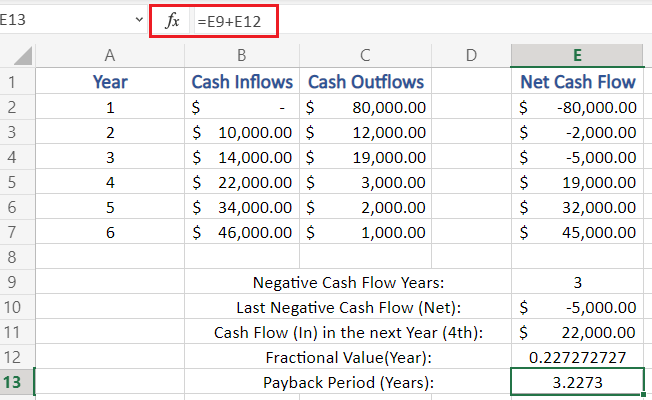
=Negative Cash Flow Years + Fraction Value
which, when applied in our example =E9 + E12 = 3.2273
This means it would take 3 years and 2 months (approx.) for our investment to capital to start giving returns.
Conclusion
That’s It! Hope you have learned well – What is Payback Period, and how to calculate Payback in Excel.
