MIRR is one of the major financial functions in Excel which is used to find out the Modified Internal Rate of Return. It can be taken from the given data of cash flows, discount rates, and rate of reinvestment. Using MIRR Function, it’s possible to calculate the modified rate of return. Hence, MIRR helps in forecasting an investment and deciding whether to go in for an investment opportunity or not.
When we go deep into this we can find some commonality between the IRR and MIRR. But the major difference is that MIRR includes both the discount rate and reinvestment rate of interest received. Hence, MIRR is widely considered as a better parameter for forecasting investments than IRR (Internal Rate of Return).
Recommended Read: IRR | How to calculate IRR in Excel
Syntax and Arguments of MIRR Function in Excel
The primary purpose to calculate the MIRR is just to find or determine the modified internal rate in the form of return. Where the return of the MIRR function is determined in the form of a percentage(%).
Syntax of the MIRR function in Excel:
=MIRR(values, finance_rate, reinvest_rate)
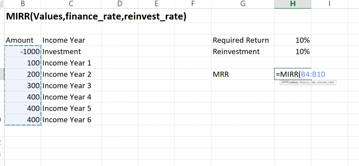
- Values = It’s the given cash flows in the table of your worksheet. Here we have assumed an amount for the different income years from B4:B10. It means it’s that reference or cells that contain the cashflows. In our case, we assumed the Table B cells as cashflows.
- Finance_rate= It’s the discount rate given in percentage form. We can also say it as the required rate of return.
- Reinvest_rate= It’s the rate of interest received from the cashflows. In any case, it may be the same as the finance_rate too.
Steps to Calculate MIRR in Excel
- Here we’ve assumed the amount, income year as shown in the image, where the amount is valued. As per the rules, the values must need to contain at least 1 negative and 1 positive value. So, we’ve set an assumption as per this.
- Also, for reference, we set both finance_rate and reinvestment_rate as the same.
Setting the Income Year
- At 1st, you can assume the time for some year. Here we have assumed income year up to 6 to determine the MIRR report till that year. In our example, it lies from C5:C10.
In the income year column, 1st cell we have entered is with Investment. This is just for making the Cashflow negative in its adjacent cells. On the other hand, it’s not necessary to write this.
Assuming the Amount for the Year
- Now, enter or assume the amount for every income year. Here we have assumed the amount of cash flow on every income year.
- For income year 1 we gave assumed the cash flow of 100. Like this, you can assume/ enter the cash flow opposite of the income year.
Finding/Assuming the required finance and Reinvest Rate
Now assume the required rate of return and reinvest rate.
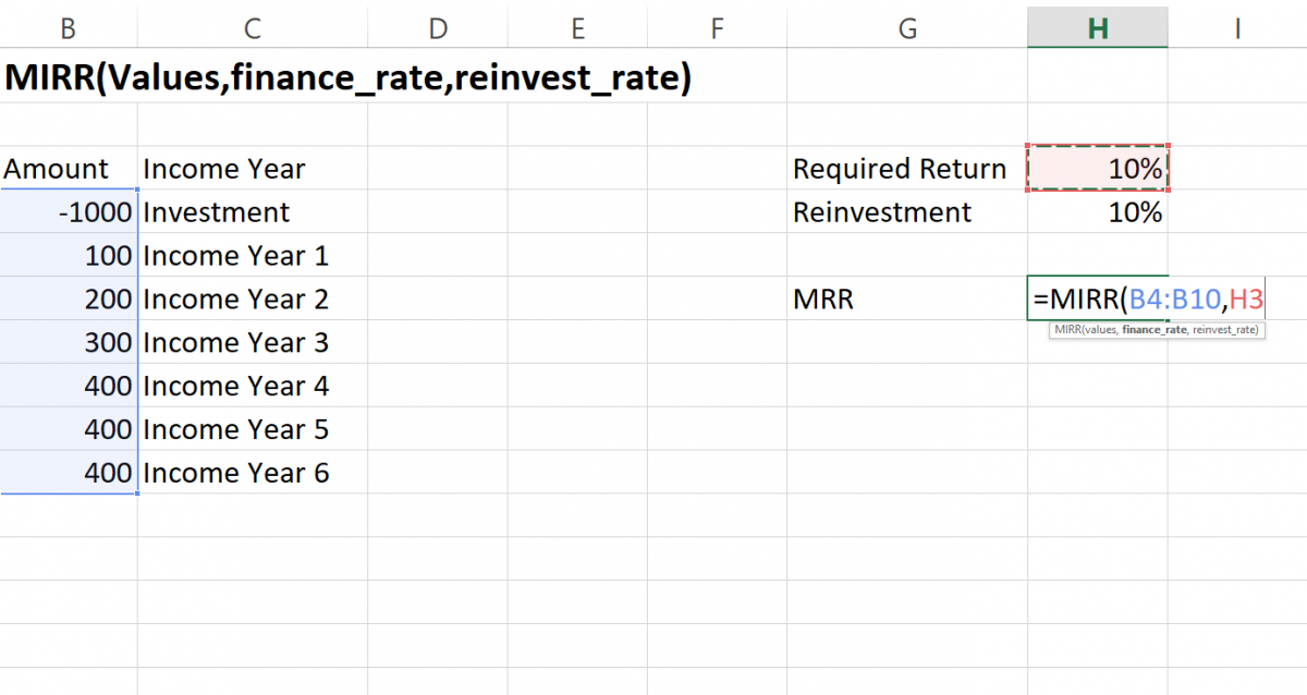
- For the required rate of return (finance_rate) we’ve assumed it to be 10%.
- For the return of cash flow (reinvest_rate), we have again assumed it to be 10% (same as of finance_rate). Here you can assume the different rate too as per your needs.
MIRR function
We put in values in the MIRR(values, finance_rate, reinvest_rate) function in Excel.
- In any cells of a blank column, type =MIRR(
- Select the values, which is cash flow. From B4:B10.
- Select the finance_rate, it’s required return which is 10%. From H3.
- Select the reinvest_rate, it’s 10%, from H4.
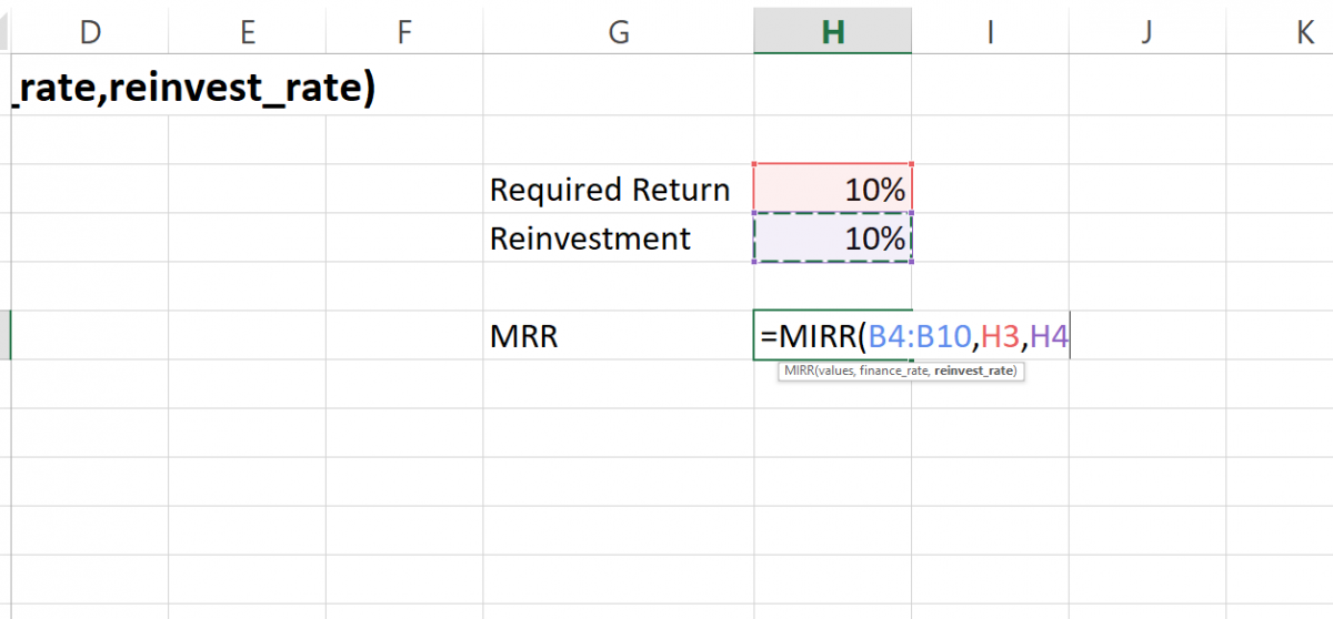
- Make sure you follow the syntax:
=MIRR(B4:B10,H3,H4)
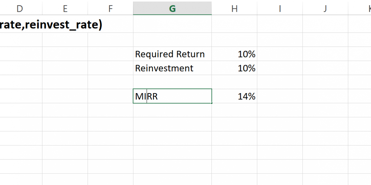
On entering the values in the MIRR function and pressing Enter, we get the final result of MIRR = 14%.
Conclusion
That’s it for the tutorial. Hope you have learned about MIRR(Modified Internal Rate of Return) and how to calculate MIRR in Excel.
