Protection is one of the major points that we consider, making our datasheets immutable. So, here we are with you to guide you on how to lock cells in Excel. Excel features on locking the cells to protect your data from being edited by another access holder. To protect the data cells here, you need to follow these simple steps.
Also read: [Step-by-Step Guide] How to Password Protect an Excel File?
By default, all the cells are automatically locked while preparing any new Excel sheet. Although these cells are locked by default, still one can edit and make changes to them. That’s where we need to protect those cells and lock them. It means at 1st we have to protect the cells using the password to lock them from being edited by anyone.
Steps to Lock Cells in Excel
Open any sheet where you want to lock cells in Excel.
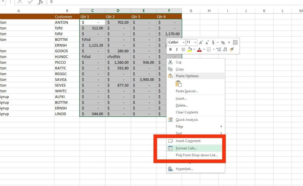
- Select the desired Cells. You can select all the cells with the help of your mouse cursor. For reference, we are selecting the cells from Qtr 1 to Qtr 4 in our sample example below
- Do a right-click, after making a selection of the specific cells.
Click on Format Cells, for this you can also press ‘Ctrl + 1‘ from the keyboard. Here we have selected the Qtr 1 to Qtr 4 from protecting with the password to lock it.
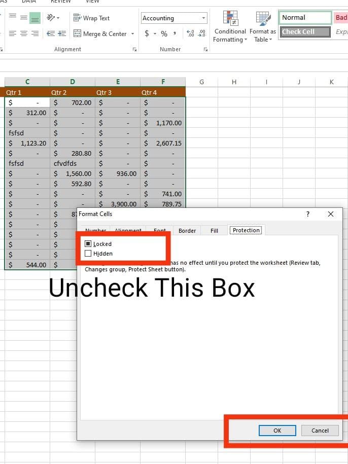
- From Format Cells go to the Protection Tab as shown in the screenshots. Here you get two options. By default, the Locked box is checked (marked with the right sign).
- Uncheck (Click on Locked to unselect it), and click on OK to save it. By default, this box is checked/ selected. So, here need to uncheck/unselect it. This will help us to protect our worksheet with password protection,
We notice the cells are still unprotected, although it’s locked by Default.
Now, as we have already selected the specific cells to lock it, so from the selection or after selecting click on the REVIEW section located on the top bar(Home tab) of Excel.
Here we have selected the Qtr1 – Qtr 4, so, make sure you have selected the desired cells before protecting them.
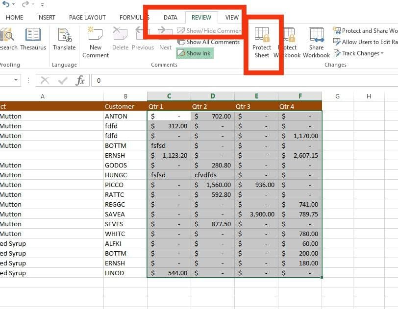
Go to Protect Sheet and Enter the Password to unprotect the sheet, here you can enter any keywords as a password, for example, 12134. Re-enter the password to proceed, i.e. 12134 in our case.
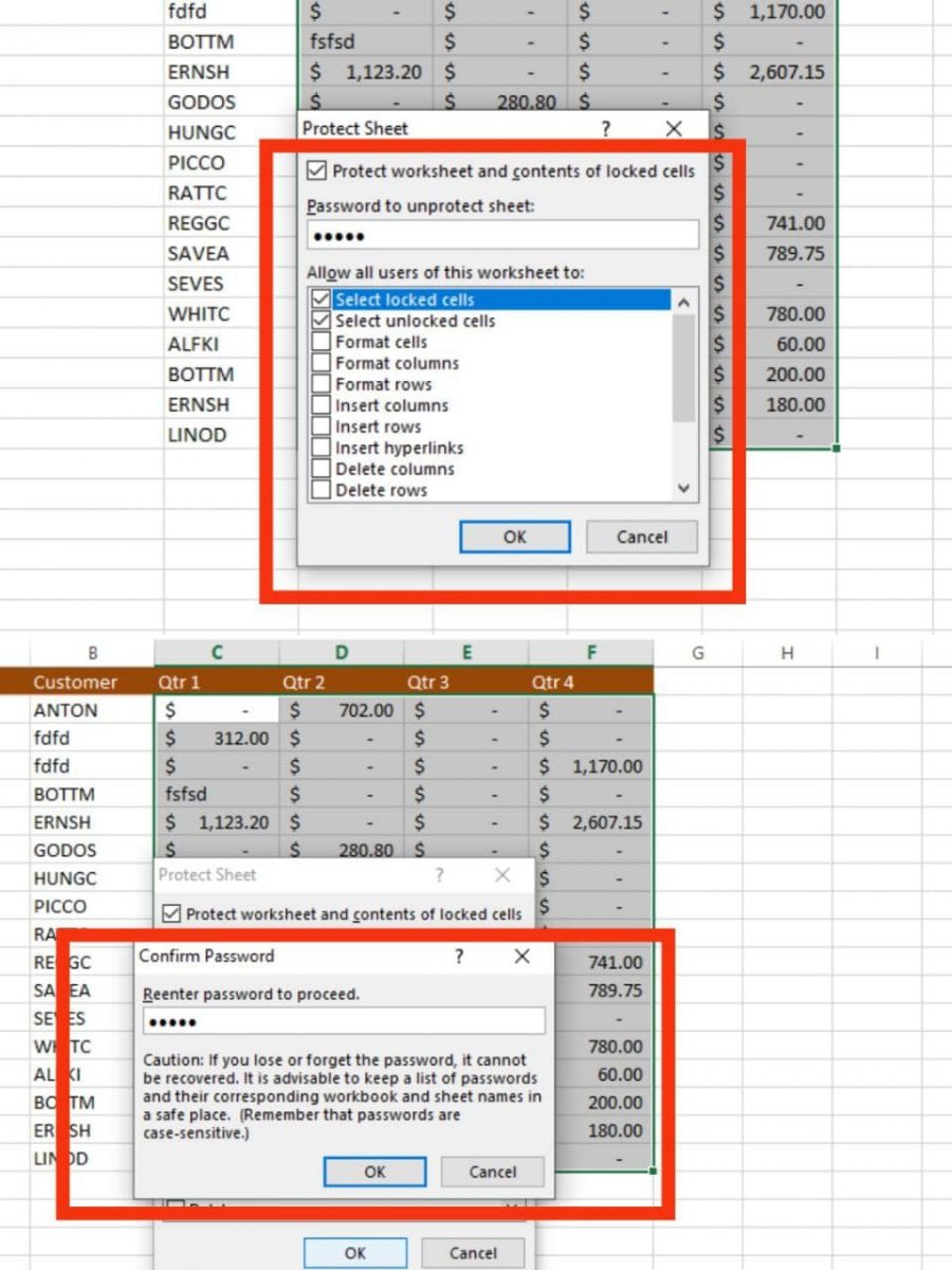
In this section, you can select the required features to allow even after protecting the sheets. You can allow some permissions for worksheets like selecting the locked cells, formatting the cells, formatting the columns, inserting hyperlinks, etc. Even after protecting the cells in Excel.
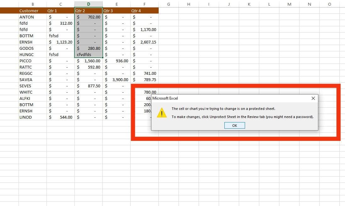
After protecting the specific cells with the password, the users are limited in editing the worksheet as per the different permissions allowed by you in the above steps.
After this, one won’t be able to edit and make changes to your worksheet. It flashes an Error message if someone tries to edit your worksheet data of the desired cells. By using these steps you can protect your data and also use the same steps for protecting All cells.
Conclusion
Here we go to the end of this Excel tutorial on How to Lock Specific Cells in Excel. Hope you have learned well and can now protect your Excel sheet from unauthorized access and edit.
