Have a spreadsheet full of data? There may be times when we’d desperately need to conceal certain entries or contents amongst the available data. This can be due to some calculations being carried out in that portion or irrelevancy of interest towards the data that is needed to be looked into. So, knowing of a way to subtly hide them is in order. We shall cover such ways available to hide cells when working on MS Excel in this article.
Listed here are the different ways of having it done.
- Using the Keyboard Shortcut
- Using the Home Tab
- The Old-School Right Click
We would be trying to hide the contents of the following table using each of the above-listed methods.
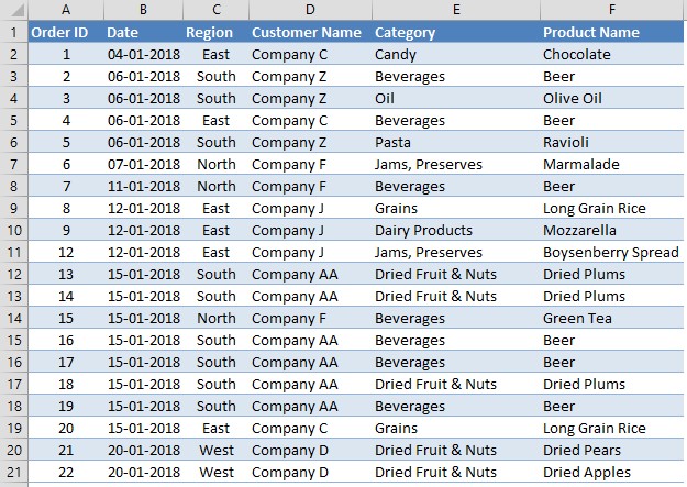
1. Using a Keyboard Shortcut
Let’s say we would like to hide the contents of Company F in rows numbers 7 & 8. First things first, we would select these cells which we need to hide as shown in the below image.
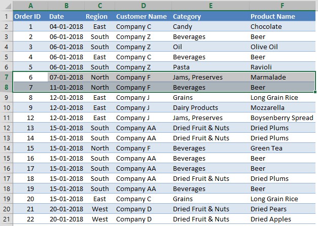
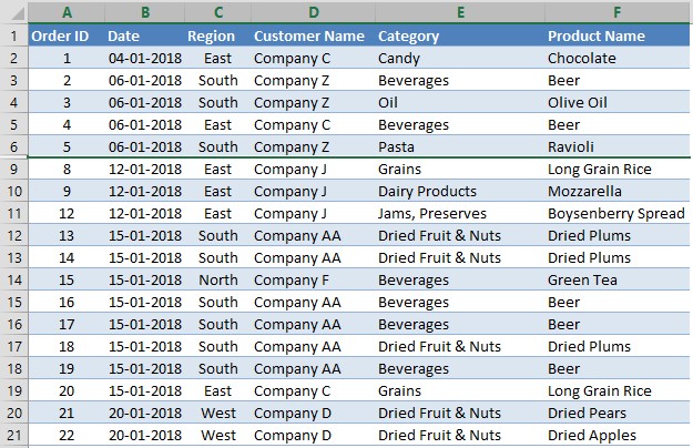
After this, we would be pressing the CTRL key followed by the number key ‘9’ (CTRL+9). The key here is to press the keys one after the other and NOT SIMULTANEOUSLY! Once done, the selected cells would be successfully hidden as shown below.
2. Using the Home Tab
The first step remains the same as in the above image, which is to select the cells that need to be hidden. We shall stick to the same cells belonging to row numbers 7 & 8 in this case. Once done, look out for the Format option in the Home tab.
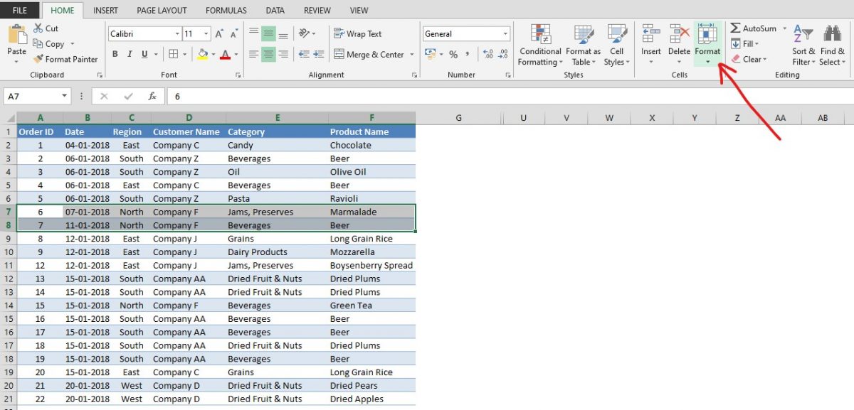
Click on Format and it shall display a list of options to choose from, but our interest here is to navigate to the Hide & Unhide option.
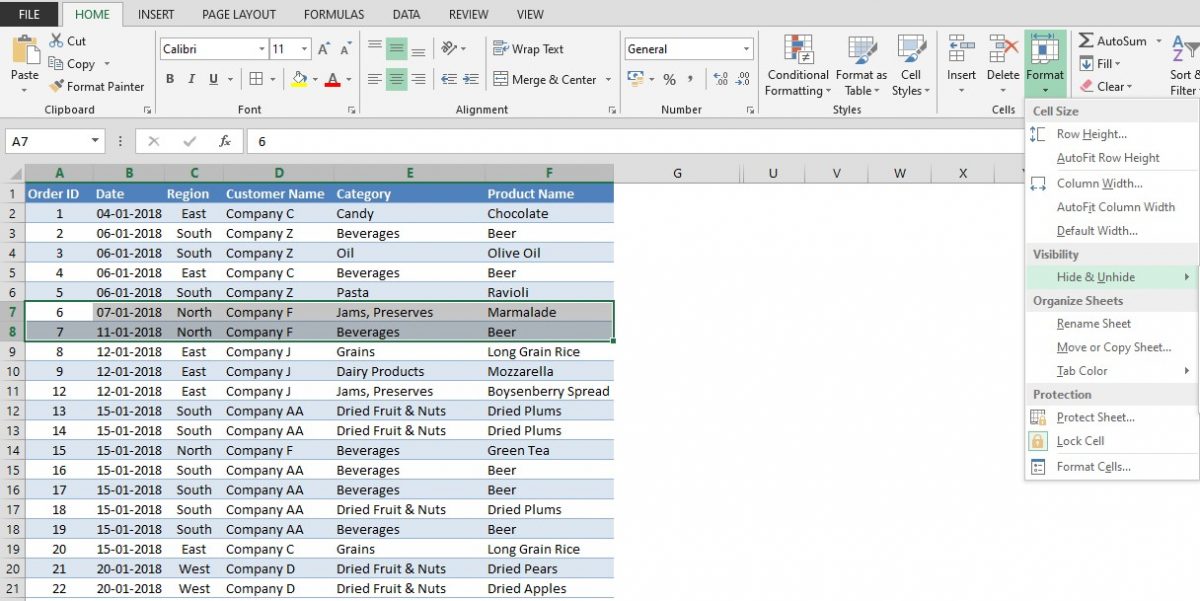
The Hide & Unhide option in turn has within itself, a list of options to choose from. Now, it is time to click on that Hide Rows option as shown below.
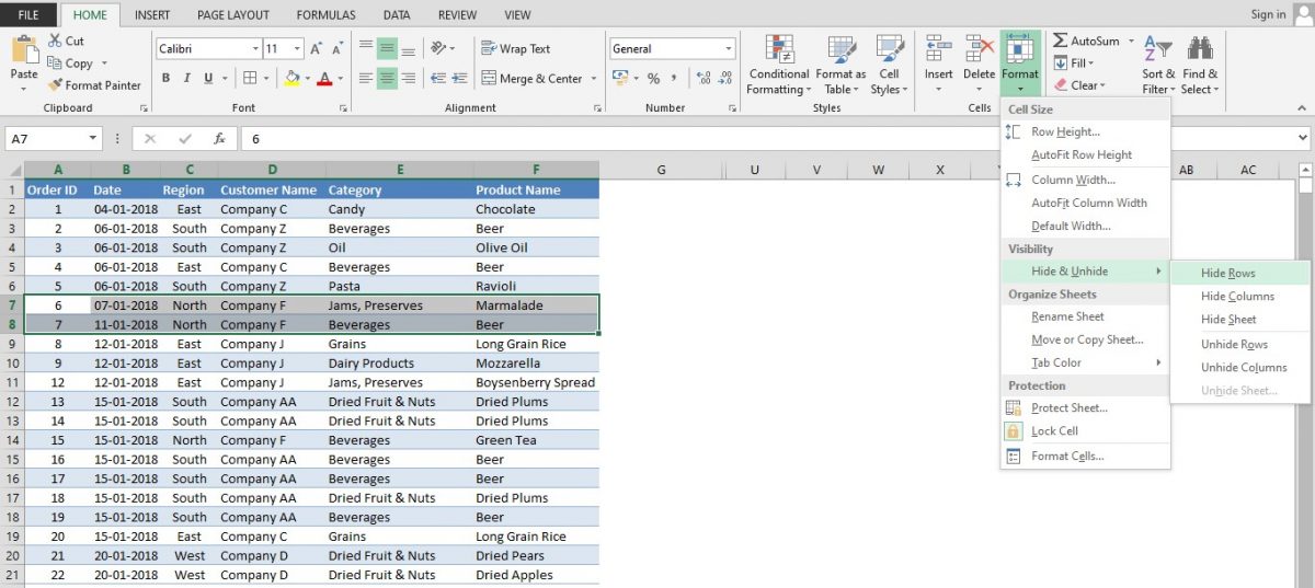
The selected contents get hidden the very moment, the Hide Rows option is clicked.

3. The Old-School Right Click
In this method, the first step is a bit different and requires a bit more than selecting the cells that are required to be hidden.
Now it is all in the mouse (for the laptop users, it’s in the mouse-pad too!) to make these selected entries hidden. Hover the cursor over the row number of the cells that are to be hidden and click that row number using your left mouse button.
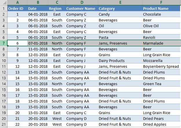
Now without lifting that finger off the left mouse button drag it one step below to select the next row number which is, Row 8 in this case.
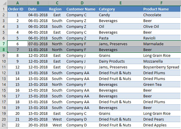
Now hover the cursor over the selected row numbers and click using the right mouse button over that space. Once done, a pallet containing a list of options to choose from appears.
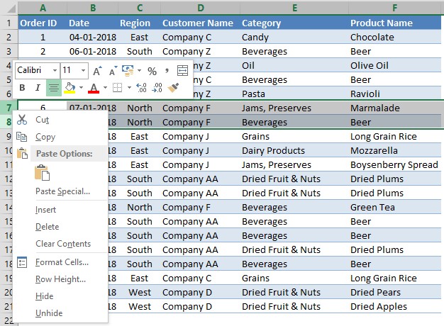
Our interest here is to select the Hide Option, in the right-click panel. Selecting that option would make the chosen cells are hidden in no time.

Conclusion:
Now that we’ve covered 3 different ways to hide the cells in MS Excel, hope it would come in handy when you face a situation of need. This article has predominantly dealt with hiding the cells across (i.e) horizontally in an active worksheet. But, there shall also arise a need to hide the cells vertically (i.e) alongside the columns in an active worksheet. That being said, check out this article, if you want to hide columns in an Excel sheet.
Do watch out for our space, QuickExcel to keep yourself updated with MS Excel. Cheers!
