How to Make a Drop-down List in Excel?

This tutorial is all about adding, removing, and managing drop-down lists in Microsoft Excel. We will learn about adding, removing, and editing existing drop-down lists via the Data validation tool in Excel.

Steps to add drop-down lists in Excel

Let’s get started with the steps to add drop-down lists in Excel.

1. Creating drop-down lists from comma-delimited lists

To insert or create a drop-down list in Excel, follow these steps.

Select the cells you want to insert drop-down lists to.
Go to the Data tab.
Under the Data Tools section, select Data Validation.
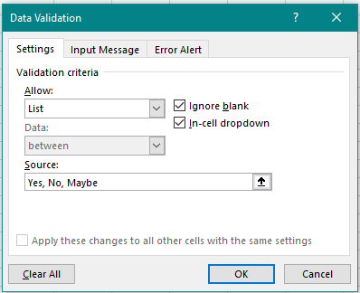
Select List under Allow.
Under Source, type the values you want to display in the drop-down list separated by commas.
This is a comma-delimited list.
Unchecking Ignore blanks will pop up an error message to the users if the cells are left blank.
Unchecking In-cell dropdown will no longer allow users to choose from a drop-down list.
Click OK to continue.

You can see that a drop-down list appears on the selected cells in Microsoft Excel.

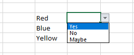
Remember that comma-delimited lists are case-sensitive in nature.

2. Creating drop-down lists from cell values in a sheet

The options in the drop-down list can be taken from multiple sources such as comma-delimited lists, values in sheets, or named ranges, etc. in Excel. Let’s learn the different ways to add list values in a drop-down list.

Select the cells you want to insert drop-down lists to.
Go to the Data tab.
Under the Data Tools section, select Data Validation.
Select List under Allow.
You can either type a comma-delimited list as we did in the previous step, or you can select the cells with values that you want to be present as the options of the drop-down list, like this.

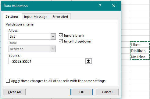
Click OK to continue.

You can now see that the selected cells can be seen as options for your drop-down list.

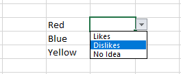
cell list enabled — Cell Values Added as List Option

Note- Any changes you make to the values in the cells that are taken as options for a drop-down list, will be reflected in the list.

3. Applying drop-down lists to other cells

To apply the same drop-down list to other cells, follow these steps.

Press DELETE on your keyboard if you have selected any option from the list.
Now press CTRL+C (Copy) on your keyboard to copy the drop-down list.
Select the cells where you want the drop-down list to be applied.
Press CTRL+V (Paste) on your keyboard.

You will find that the drop-down list has now been applied to other cells as well.

4. Creating drop-down lists from a named range

When a cell range is named, it is called a named range.

You simply name a range by selecting the range of cells.
Set a name in the Name Box (highlighted in Yellow in the image below)
A range name can start with a letter or an underscore “_”.
The rest of the name can be a “.”, letters, underscores “_” or even numbers.
You cannot add spaces to a name.
Or cannot add predefined statements like True or False or cannot have cell references as the range name such as B32.
We have named our cell range as List_Options, for instance.

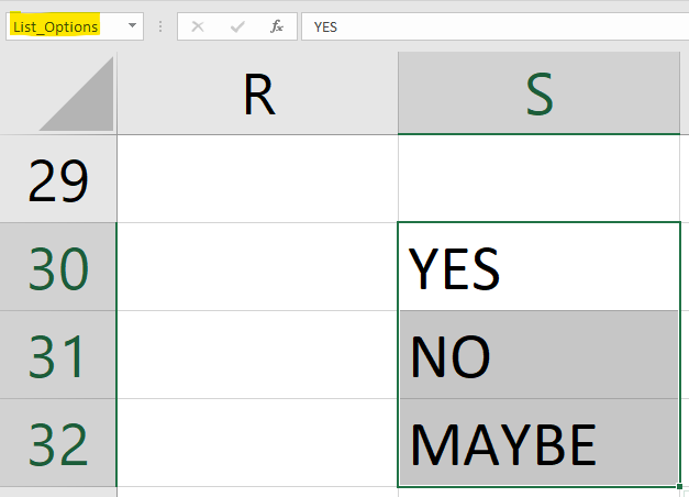
Let’s continue to create a drop-down list in Excel using a named cell range.

Select the cells you want to insert drop-down lists to.
Go to the Data tab.
Under the Data Tools section, select Data Validation.
Select List under Allow.
Click the Source dialogue box.
Press F3 or Fn+F3 on your keyboard to select the named range.
A window named Paste Name opens.
Choose the name you set for your range and click OK.

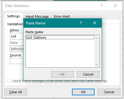
Click OK again to apply the changes.
Copy the drop-down list to the other cells as mentioned above.

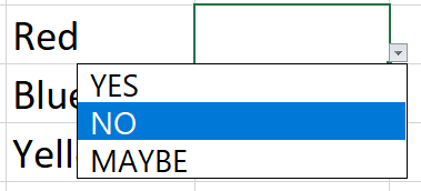
named range applied — Named Range Added as List Options

You can now see that the drop-down list displays the cell values of the named cell range.

5. Error alerts and input messages for dropdown lists

The Input Message option in Data validation is used to pop up a message to notify users that there is a dropdown list in the cell. Here’s how to do it.

Select the cells you want to add a message to.
Go to the Data tab.
Select Data Validation.
Under the Input Message tab, check the box that says Show input message when a cell is selected.
Set a custom title for the input message (optional).
Set a custom input message to display to users (optional).
Click OK when you’re done.
Uncheck the box to stop displaying input messages.

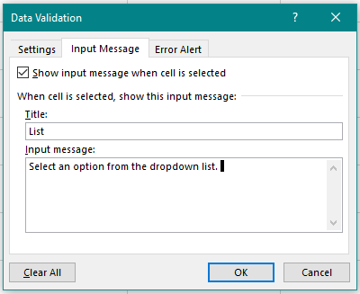
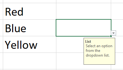
message displayed — Input Message Displayed

You can see that the input message is being displayed to the users.

You can even set error alerts for users whenever an invalid entry has been made. Meaning, if a user types an option that is not present in the dropdown list, you can choose to display an error alert to the user. Here’s how to do it.

Select the cells you want to add a message to.
Go to the Data tab.
Select Data Validation.
Under the Error Alert tab, check the box that says Show error alert after invalid data is entered.
Select a style of alert under the Style section.
Set a custom error title that should be displayed.
Click OK to continue.
Uncheck the box to stop displaying error alerts.

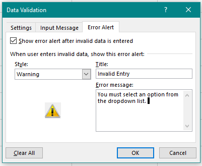
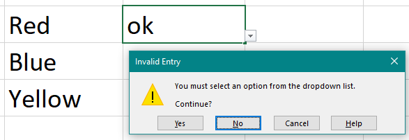
You can see that the error alert is being displayed when an invalid entry has been entered.

Also read: How to Hide or Unhide Columns in Excel?

6. Removing dropdown lists in Excel

To remove or clear all existing dropdown lists, do as follows.

Select the cells with dropdown lists inserted on them.
Click Data Validation.
Click Clear All to remove all dropdown lists.
Click OK to continue.

Clear All Button

Also read: How to Password Protect a Sheet in Excel?

Conclusion

This article was all about creating, removing, and managing dropdown lists in Excel. Follow these steps carefully to be able to successfully add or remove dropdown lists in Excel. Feel free to comment below if you have any doubts regarding dropdown lists!

Reference: Microsoft