A straight line is not always the best method to fit your data points. For these specific cases, we can use some of the tools available in Excel to do nonlinear regression or curve fitting.
Methods to Perform Curve Fitting in Excel
Without any further ado, let’s get started with performing curve fitting in Excel today. We’ll explore the different methods to do so now.
1. Polynomial Curve Fitting Model
Let’s consider some data points in x and y, we find that the data is quadratic after plotting it on a chart. A polynomial function has the form: y = ax2+ bx + c
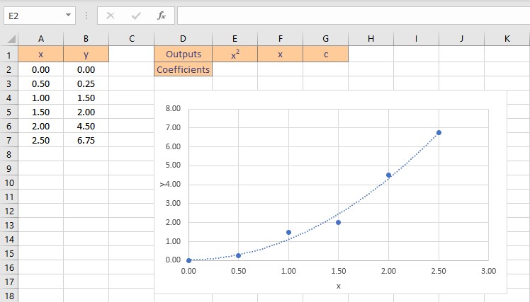
Although this data is nonlinear, the LINEST function can be utilized to obtain the best fit curve. We can return the coefficients straight to cells when we use LINEST to acquire the coefficients that define the polynomial equation.
There are three coefficients, a for x squared, b for x, and a constant c since the equation is quadratic, or a second-order polynomial. Follow these steps to obtain the coefficients a, b and c:
- Select the cell where you want to calculate and display the coefficients.
- Type the formula =LINEST(y, x^{1,2}, TRUE, FALSE), where y is the cells containing the known y data and x is the cells containing the known x data raised to the first and second power. Finally, the TRUE and FALSE parameters instruct the LINEST function to calculate the y-intercept without forcing it to zero and not to return further regression data, respectively.
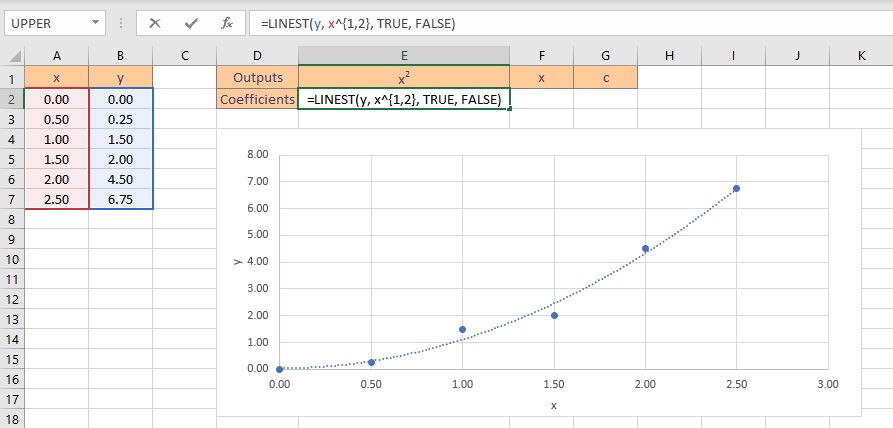
- Press the Ctrl+Shift+Enter keys to return the result.
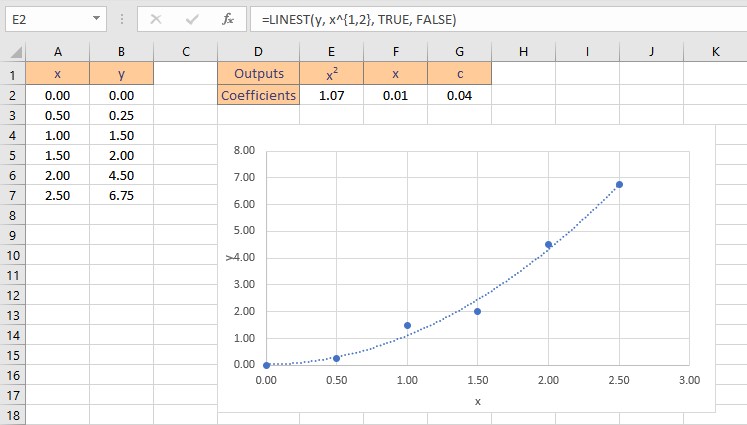
Therefore, the polynomial curve fitting formula for the given dataset is: y = 1.07x2+ 0.01x + 0.04
2. Logarithmic Curve Fitting Model
Let’s consider some data points in x and y, we find that the data is logarithmic after plotting it on a chart. A logarithmic function has the form: y = m.ln(x) + b
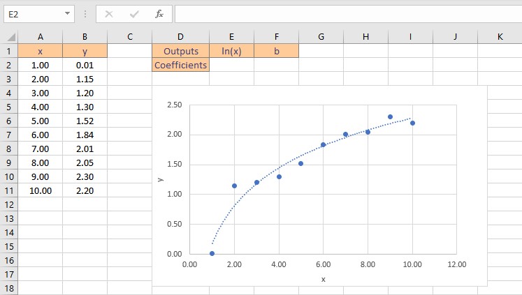
Although this data is nonlinear, the LINEST function can be utilized to obtain the best fit curve. We can return the coefficients straight to cells when we use LINEST to acquire the coefficients that define the logarithmic equation.
There are two coefficients, m for ln(x) and a constant b. Follow these steps to obtain the coefficients m and b:
- Select the cell where you want to calculate and display the coefficients.
- Type the formula =LINEST(y, LN(x), TRUE, FALSE), where y is the cells containing the known y data and x is the cells containing the known x data. Finally, the TRUE and FALSE parameters instruct the LINEST function to calculate the y-intercept without forcing it to zero and not to return further regression data, respectively.
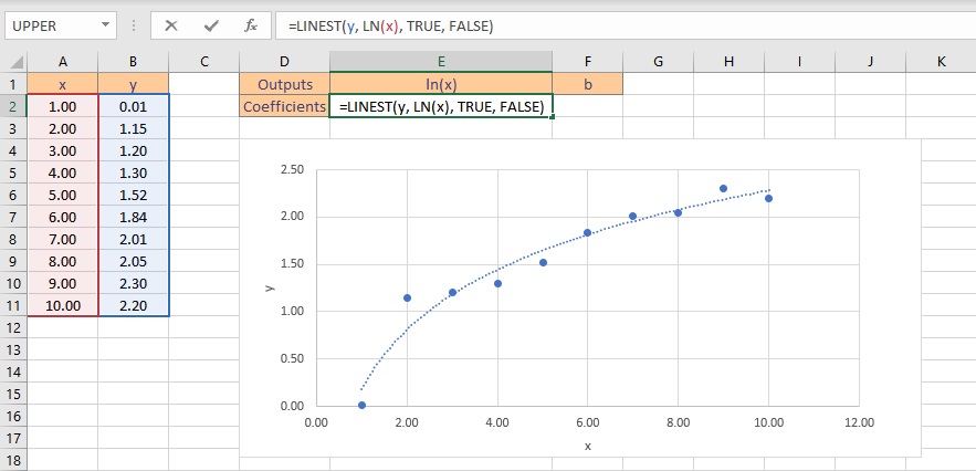
- Press the Ctrl+Shift+Enter keys to return the result.
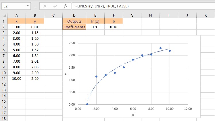
Therefore, the logarithmic curve fitting formula for the given dataset is: y = 0.91ln(x) + 0.18
3. Exponential Curve Fitting Model
Let’s consider some data points in x and y, we find that the data is exponential after plotting it on a chart. A logarithmic function has the form: y = aebx
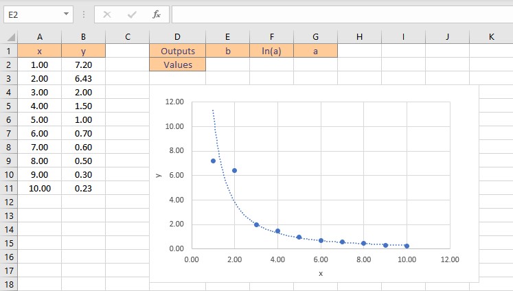
It’s a little more difficult to find the coefficients, a and b, for this equation since we need to do some algebra first to make the equation take on a “linear” form. To begin, compute the natural log of both sides of the equation to obtain the following: ln(y) = ln(a) + bx.
We can now use LINEST to get ln(a) and b by entering ln(y) as the y values argument using the formula =LINEST(LN(y), x, TRUE, FALSE). From ln(a), we can simply apply the exponential function to get just “a” as a = eln(a) . Follow these steps to obtain the coefficients a and b:
- Select the cell where you want to calculate and display the coefficients.
- Type the formula =LINEST(LN(y), x, TRUE, FALSE), where y is the cells containing the known y data and x is the cells containing the known x data. Finally, the TRUE and FALSE parameters instruct the LINEST function to calculate the y-intercept without forcing it to zero and not to return further regression data, respectively.
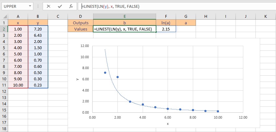
- Press the Ctrl+Shift+Enter keys to return the result for b and ln(a).
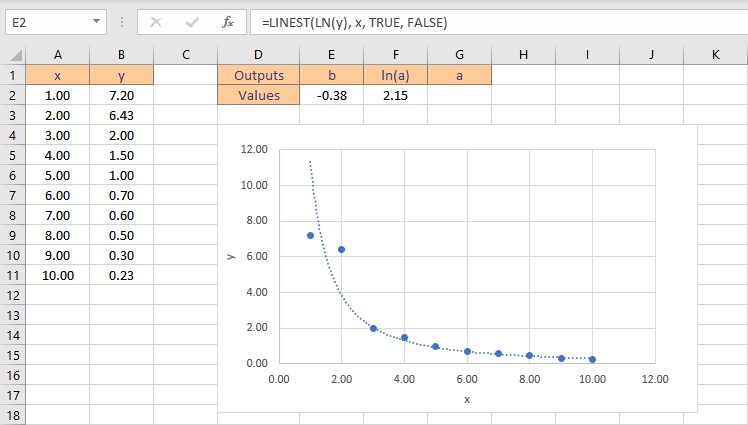
- To get the value of a, type =EXP(F2), where cell F2 contains the value of ln(a).
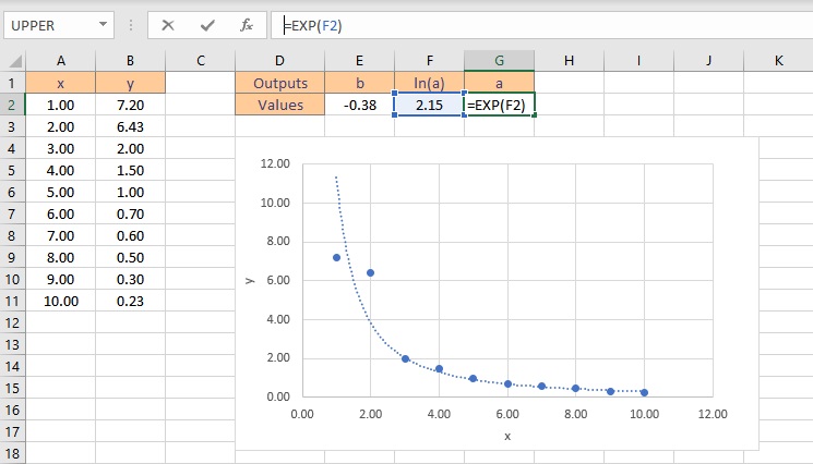
- Press the Enter key to display the result.
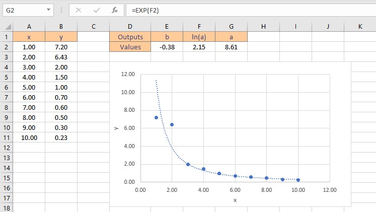
Therefore, the exponential curve fitting formula for the given dataset is: y = 8.61e-0.38x
4. Power Curve Fitting Model
Let’s consider some data points in x and y, we find that the data is in power model form after plotting it on a chart. A power function has the form: y = axb

It’s a little more difficult to find the coefficients, a and b, for this equation since we need to do some algebra first to make the equation take on a “linear” form. To begin, compute the natural log of both sides of the equation to obtain the following: ln(y) = ln(a) + bln(x). We can now use LINEST to get ln(a) and b by entering ln(y) as the y values argument and ln(x) as the x values argument using the formula =LINEST(LN(y), LN(x), TRUE, FALSE). From ln(a), we can simply apply the exponential function to get just “a” as a = eln(a). Follow these steps to obtain the coefficients a and b:
- Select the cell where you want to calculate and display the coefficients.
- Type the formula =LINEST(LN(y), LN(x), TRUE, FALSE), where y is the cells containing the known y data and x is the cells containing the known x data. Finally, the TRUE and FALSE parameters instruct the LINEST function to calculate the y-intercept without forcing it to zero and not to return further regression data, respectively.
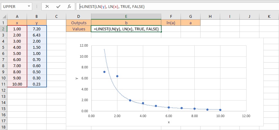
- Press the Ctrl+Shift+Enter keys to return the result for b and ln(a).

- To get the value of a, type =EXP(F2), where cell F2 contains the value of ln(a).
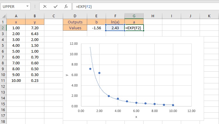
- Press the Enter key to display the result.
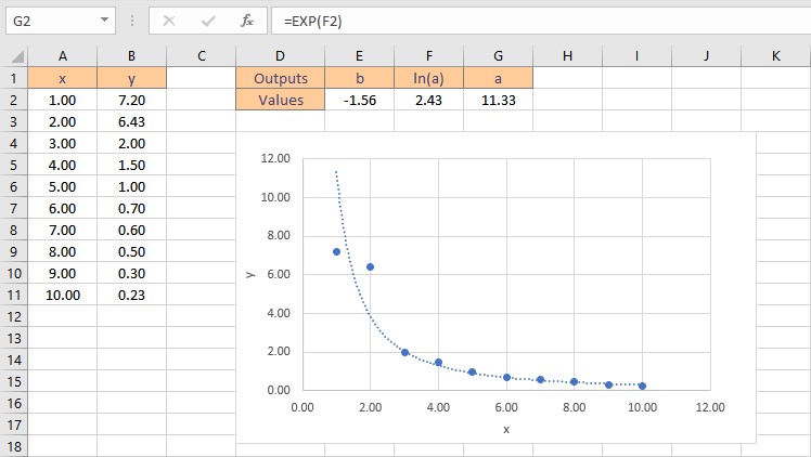
Therefore, the power function curve fitting formula for the given dataset is: y = 11.33x-1.56
Conclusion
In this tutorial, we learned how to perform curve fitting In Excel using different models.
