We would all have gazed at the skies & tried to count the stars at least once in our life. Counting seems to be an obsession for humanity and that explains the origin of sayings such as ‘Don’t count your chickens before they hatch!’.
We always need to have track of things & counting them is the first step toward that. In this article, we would be diving deep into the greater depths of using a conditional counting statement in MS Excel – the COUNTIF.
COUNTIF Syntax:
We shall first understand what this formula is made of by looking into its syntax,
=COUNTIF( range, criteria )
Where,
- range – the series of cells which is to be counted based on a condition
- criteria – the condition to count
Using COUNTIF:
While selecting the ‘range’ may be a straightforward aspect, one can flex the COUNTIF to suit different requirements using its ‘criteria’. Following are the types of criteria that can be used for constructing this formula.
- Numerical Criteria
- Double Quoted Criteria
- Logical Criteria
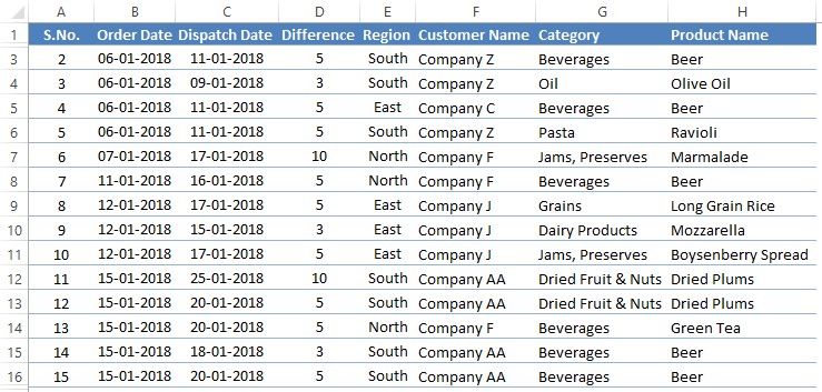
The following dataset shall be used to demonstrate how to frame each of the above criteria.
Numerical Criteria –
The criteria is directly typed within the formula so that it counts all the cells containing that particular number in the selected range.
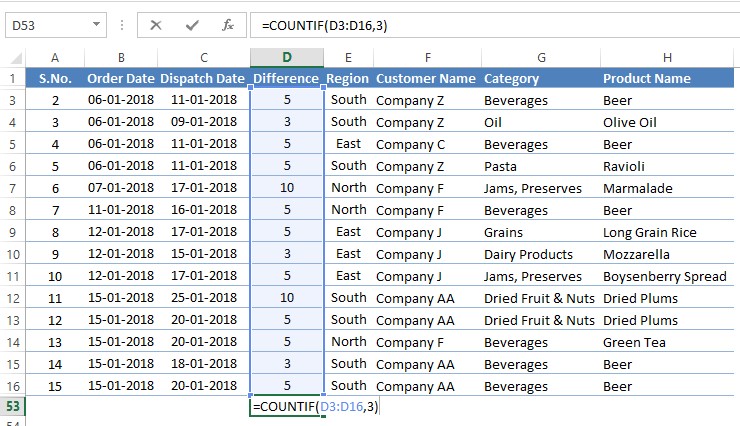
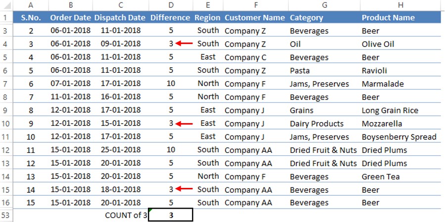
The formula constructed in the above image counts the number of times ‘3’ occurs in the selected range & here’s the result.
Double Quoted Criteria –
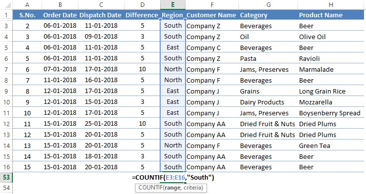
All the other types of data that ought to be counted, but without the inclusion of any logical operators fall into this category. The double quotes (“ “) are being used here to tell MS Excel not to misinterpret these into some incomplete formula nested within COUNTIF.
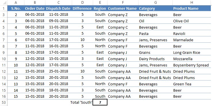
For instance, to count the number of ‘South’ under the Region column, the formula shall be constructed as shown below.
Hit ENTER & the result shall appear.
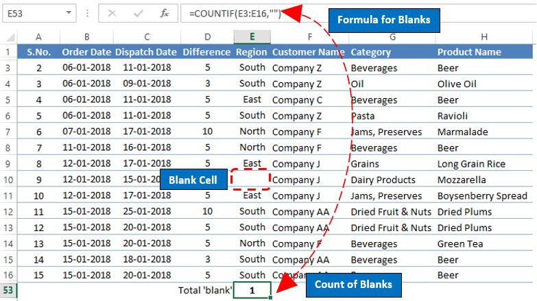
One can also count the number of blank cells in a selected range by placing just the double quotes in the criteria without any spaces(‘””).
Formula to count blanks =COUNTIF(cell range, “”)
Let’s try counting the number of blank cells under the Region column.
Logical criteria –
COUNTIF also helps us to analyse whether the data within the selected range is greater than (>x), less than (<x) or not equal to (<>x) a specific data. All these logical statements are to be put within double quotes while being typed as the criteria for the COUNTIF formula.
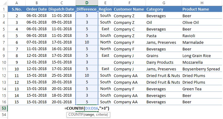
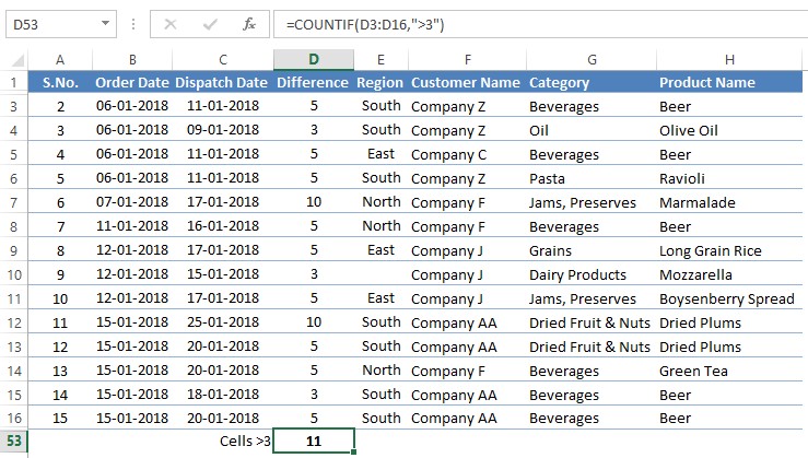
So, let us get on with constructing a formula for each of these categories and see how it works. For counting cells greater than 3 in column D, one has to give the criteria as “>3” as shown below.
Hit ENTER & the result is displayed.
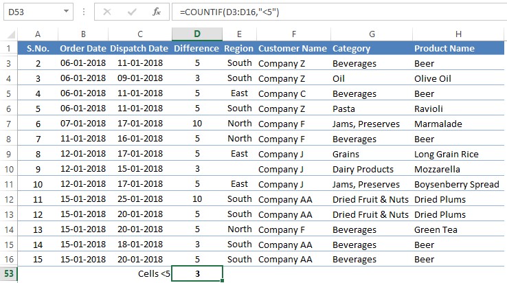
For counting cells lesser than 5 in column D, one has to give the criteria as “<5” in a similar manner as given below.
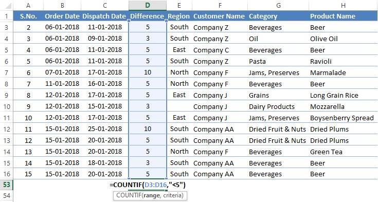
Hit ENTER & the result is displayed.
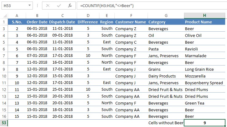
For counting cells that do not contain ‘Beer’ under the column Product Name the COUNTIF formula shall be constructed with the criteria as “<>Beer”. One has to bear in mind that COUNTIF ain’t case sensitive. So, be it ‘Beer’ or ‘beer’ or ‘BEER’, everything is the same to COUNTIF & it shall treat all the variations as the same.
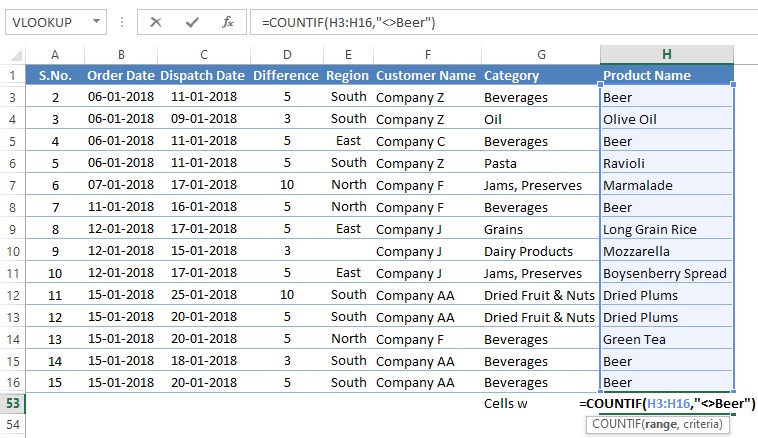
Hit ENTER & the result shall appear as shown below.
Conclusion:
Now that we have reached the end of this article, hope it has elaborated on the different applications of putting the COUNTIF formula into use. Here’s another article which details how to count duplicates in MS Excel. There are numerous other articles too in QuickExcel that can come in handy for those who are in looking to level up their skills in MS Excel. Cheers!
