All the rows and columns in the spreadsheet not only contain data in form of text or numbers, but at times we would be needing to play around with colours to make them more appealing visually. So, that leaves us wondering whether we’d be able to perform some computations using these colours & the answer is YES!
Why should numbers have all the fun?
Why not colours?
MS Excel extends its capability to perform a number of tasks using colours as well. In this article, we would be exploring a way to count the coloured cells.
We’d be using the following dataset to count its coloured cells.
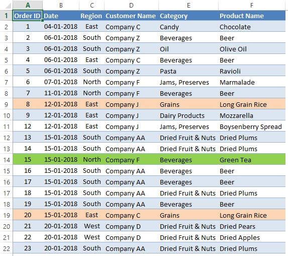
Filtered Sub-Totalling Method:
In this technique, one would be combining two different commands & putting them into use to get to know the count of cells for each colour. So, let’s get to find out how this can be done.
It all starts with applying a Filter to the header row, which in this case is row 1. Select all the contents of row 1 as shown in the below image.
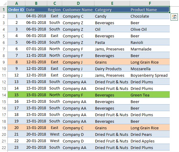
Once done, select the Filter option within the Home tab by clicking on the Sort & Filter group as shown in the below image.
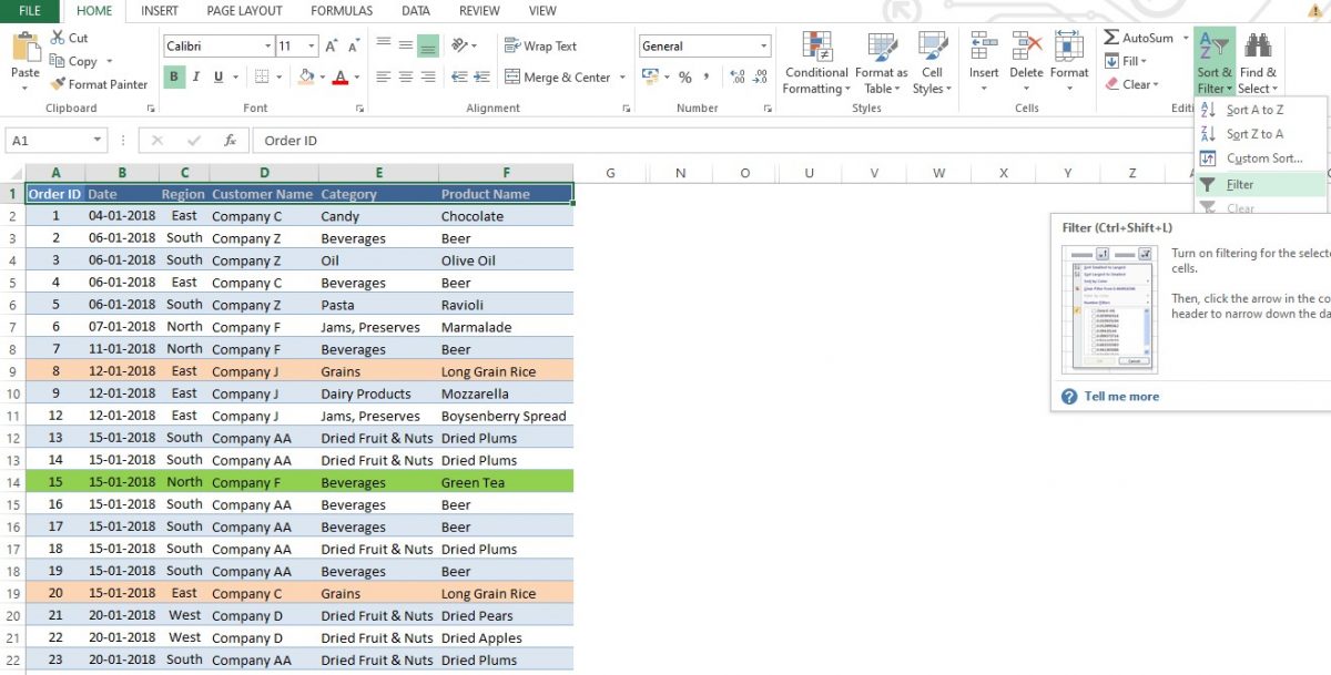
For those who are fond of keyboard shortcuts, the same can be done by pressing CTRL, SHIFT & L keys one after the other. Much emphasis here on not pressing the keys simultaneously!
CTRL + SHIFT + L
Carrying out either of the above-mentioned ways would result in the filters getting applied to the headers as shown in the below image.
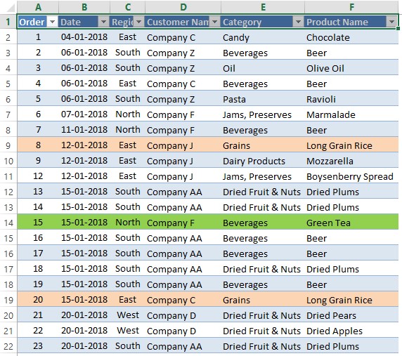
We’re now halfway through after having applied the filters & will now get to the part where we count the coloured cells – SUBTOTAL!
One can always go & search within the Formulas Tab to select this formula for usage. But before that, choose the column whose coloured cells are to be counted & then click on the cell below the bottom of the dataset to make it the active cell.
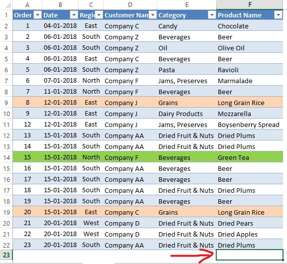
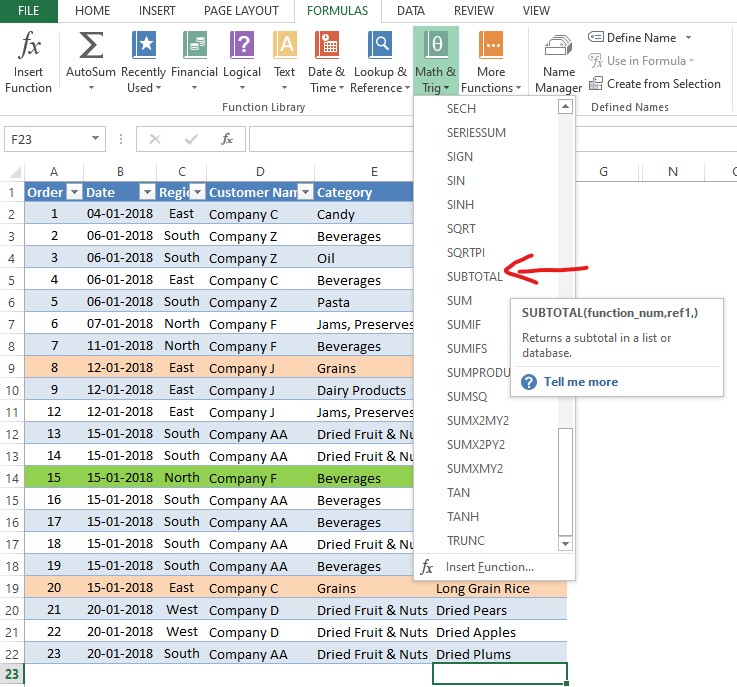
Now it’s time we summon SUBTOTAL for action and one can do that by selecting the SUBTOTAL option available under the Math & Trig category of the Formulas tab as shown in the below image. This can also be done by typing SUBTOTAL with an EQUALS (=) sign in the beginning to construct the formula.
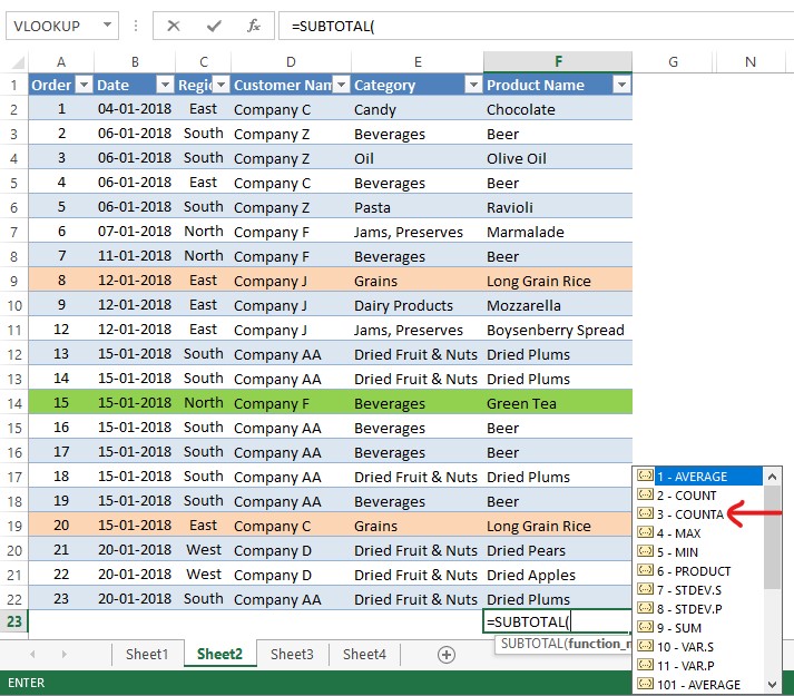
After the selection, the following list of options would appear to choose the function which we would like to perform using the SUBTOTAL. Here, our intent is to count the non-empty cells & so we choose 3 – COUNTA.
Then, the entire cells in the column are chosen.
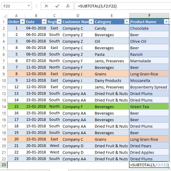
Hit ENTER & the total count of entries in the selected range shall appear.
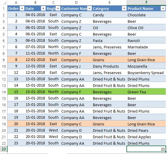
It all comes down to the filtering to count the total cells of a selected colour. For instance, we select green using the filter on the Product Name as shown below.
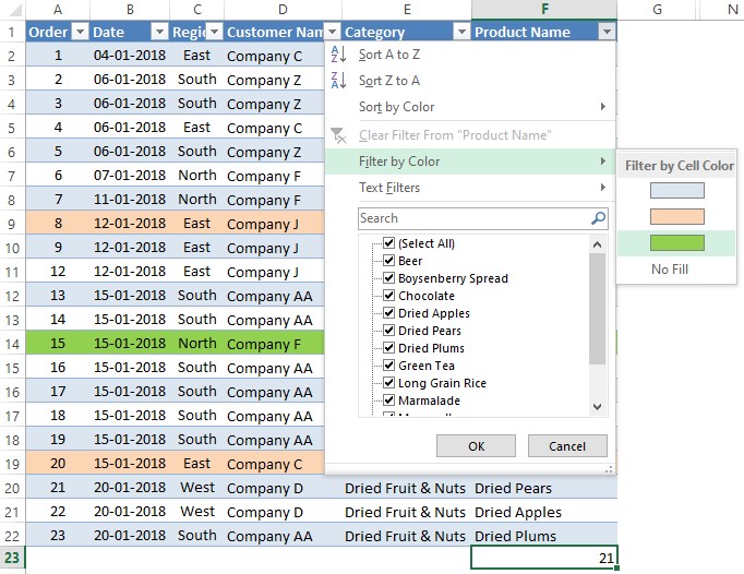
The moment the green colour is clicked, the filter gets applied & only the cells containing the green colour are now displayed along with the count of cells at the bottom.

Conclusion
Likewise, the same filtering can be done for the other colours as well & the total count of cells with that colour would be displayed at the bottom. Hope the article was informative. Do have a look at this article, to know how to count a range of cells using MS Excel. QuickExcel also has numerous other articles, which could help you in many ways to use MS Excel. Ciao!
