Data is not always about numbers with comma separators. Sometimes, it could be a text describing something or sometimes, it could be a day or a month or a year indicating the occurrence of a certain activity. It is common sense that numbers can be subjected to all sorts of arithmetic, but what about dates? Ever wondered how the values of dates could be used while calculating in MS Excel?
If that very thinking leaves you intrigued, we shall drill down deep in this article on the usage of dates in two different columns to extract the difference between them in days. The dates that are given under the Order Date & Dispatch Date columns of the following tabulation will be used for the demonstration.
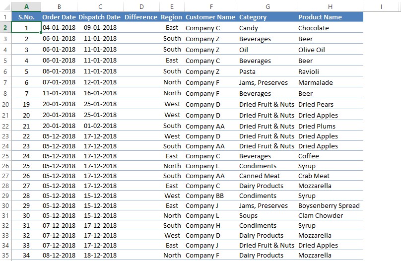
Each of the below techniques shall be used for calculating the difference in days.
- Method I – Operand Way
- Method II – DAYS Formula
Method 1 – Operand Way:
This technique is quite straightforward! It makes use of the underlying principle deployed by MS Excel to record the values of dates. The key is in the details where the date might appear with the DD-MM-YYYY format or any other chosen format for that matter, deep underneath MS Excel assigns a value to this date.
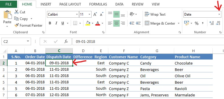
The following example will help you understand better where we are going to select a date & change its format to have a look at the numerical value assigned to it. Let us select cell C2 for instance & click on the dropdown button as indicated in the image below.
Select the Number option from the dropdown list as shown below.
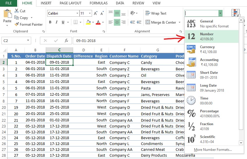
Once the option is chosen, the date which was displayed earlier in cell C2 is now turned into its numerical equivalent.

What we could infer from this is that the dates are just numbers underneath & just like numbers we can find the difference between them by subtracting the one from the other. That’s exactly what we would be doing!
Change the cell from the Number format back to the Date & move the active cell to D2.

Once done, type an equals sign (=) followed by selecting the dispatch date in C2.

Type a minus sign (-) after C2, followed by selecting the order date in B2.

Hit ENTER & the difference between the two selected dates shall be displayed in cell D2.

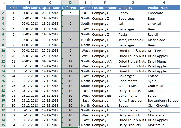
The same formula can be copied & pasted into all the subsequent cells below to determine the difference between the dispatch dates & the order dates throughout.
Method 2 – Days Formula:
This method would be delivering exactly the same result but making use of an in-built formula instead of constructing one from scratch. After making D2 as the active cell, type an equals sign (=) followed by DAYS as shown below.

Hit the TAB key now & an open parenthesis shall appear after DAYS.

Now we shall select the constructs of the formula by selecting the end date first.

Place a comma (,) after C2 & select the start date.

Include a closing parenthesis after B2 & we’re done! Hit ENTER & the difference between the selected dates will be displayed.

Copy the formula & paste it to all the cells below in order to calculate the difference across the tabulation.
Conclusion:
Hope the article was informative and you have got what you were looking for! There are also numerous other articles in QuickExcel that might come in handy for those who are in a quest to know something more in MS Excel. Cheers!
