Compound interest is considered one of the wonders of the mathematical world. It is the interest that you earn on the interest of the previous period. Interest-ception, maybe? Well, for people interested in personal finance, you know the value compound interest adds to your financial lives. Today, we’ll build a compound interest calculator in Excel so you can keep track of your investments and their future returns right on your Excel file.
While many have heard of compound interest, you may not know the exact formula to calculate the compound interest. So let’s get started with that first.
What is Compound Interest?
Compound Interest is the method of addition of interest to a loan or deposit after a set time period to the principal amount or previous ended time period’s ending amount.
The Formula to Calculate Final Compounded Amount is:

Where:
A = Final Amount
P = Principal Amount (Initial)
r = Interest rate
n = number of times interest is applied per time period or number of times the amount is compounding
t = number of time periods or years
Here’s the formula to get the compound interest:
C.I. = A(Final Compounded Amount) — P (Principal Amount)If you don’t quite get it yet, that’s alright. Let’s explore this further with an example.
Example for Compound Interest
Assume Jason invested $10,000 in a Government Railway Bond for 5 years. The compounding frequency for this bond is 6 months, which means the interest amount is accumulated every 6 months. And the rate of interest for this bond is 10%.
So we have:
P = $10,000, r = 10% per year, t = 5 years and n = 2 times (as 2 half-years in a year)
So his statement in 5 years will look like this:
| Year | January – June | July – December |
|---|---|---|
| 1st Year (2021) | $10,500.00 | $11,025.00 |
| 2nd Year (2022) | $11,576.25 | $12,155.06 |
| 3rd Year (2023) | $12,762.82 | $13,400.96 |
| 4th Year (2024) | $14,071.00 | $14,774.55 |
| 5th Year (2025) | $15,513.28 | $16,288.95 |
From the above statement, it is evident that in the duration of 5 years, Jason’s investment appreciated to $ with a Compound Interest of ($16,288.95 – $10,000 ) = $ 6,288.95
Note: I have used r = 10% for simpler calculations.
Calculate Compound Interest in Excel
As you now have a better idea of what compound interest is, how it is calculated, and what kind of information you need as inputs, let’s plot this out on our Excel sheet.
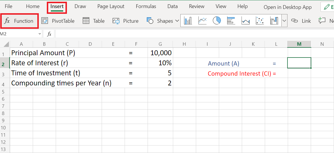
Step 1: Navigate to “Function”
- Select a cell where you want to display your result
- Navigate to ‘Insert‘ and then click on ‘Function‘

Step 2: Create a “Compound Amount Function”
- Choose create a function on the popup window
- If creating a function isn’t available as a direct option then click on any other function [here we have clicked on ‘Sum’ function]

- Then clear everything after the Equal sign (=) [ Notice the function bar]

- Start substituting values in the formula of Compounded Amount (A) given here.
Formula to calculate Amount (A) = P* (1+(r/n))^(n*t)

So here you get the final answer of Amount (A) = $16, 288.95
Step 3: Create a Compound Interest Function
To get the result of Compound Interest (C.I.) – Follow the above steps,
- Create a function of Compound Interest
- Substitute values in it to get the result
Formula to Calculate Compound Interest (C.I.) = A (Amount) – P (Principal)

Hence, we find the Compound Interest for the given data is = $ 6,289
Conclusion
That’s it! We have our own compound interest calculator. You can add the absolute returns that you’ve earned over the same period by calculating the percentage right below the compound Interest amount.
We hope you learned and enjoyed this lesson and we’ll be back soon with another awesome Excel tutorial!
