In this article, we’ll calculate ARR in Excel. Accounting Rate of Return is one of the calculation percentages of the rate of return, particularly relevant in long-term investments. If you are planning to invest in a long-term project, then it’s necessary to check out the possibilities of the return from this benchmark percent.
So, it’s the best concept for computing the potential of the possibility of getting the percentage of return in this challenging financial environment.
In simple terms, it’s the return of investment and the way to whether to accept or not. Calculating the ARR in Excel is an easy task, with the help of Salvage Value, we can find out whether the project is to be accepted or not meaning the product/commodity is worth investing in or not. Besides this, we also need to have an Average EADT, NCO for calculating the ARR in Excel.
Steps to Calculate ARR in Excel
ARR is the combination of an Average Annual Profit by Average Investment. Symbolically,
ARR = Average EADT/ (NCO + Salvage Value/2)
Using the spreadsheet it’s easy to track out the easy changes in the ARR. So, check out the steps to keep on calculating the ARR in Excel.
1. Creating the Year Date
At 1st, we need to create the date of a specific year. Also, you can assume the date for some years. Here we have assumed the time to be 6 years from cell A6:A11.
Assuming the data up to certain years gives an idea about coping with the challenges and rate of return from that investment.
2. Create CFAT Data
After assuming the project for a defined year, enter the CFAT Value of each year. Here for Year 0, we have entered the CFAT Value of (100000).
Enter the CFAT Value for all the assuming years. We have entered the value for all the years assumed.
3. Create EADT
Assume the different values for different years in EADT Column. Earnings After Depreciation and Taxes (EADT) for each year. Since Year 0 cannot earn any return, we’ve placed an empty value.
Enter an assuming or given EADT value for each year. We have entered the EADT value for all except the Base Year (Year 0) and Final Year (Year 6).
4. Calculate an Average EADT
To calculate the average of EADT, choose a cell for the result, here we have chosen another column cell to calculate an average.
Enter the syntax of Average, and select the EADT Column cells. It’s =AVERAGE(C6:C11).
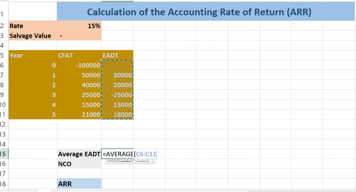
Here you will get an Average EADT.
5. Calculation of NCO Value
Type, =SUMIF(range,criteria,(sum_range)
Select the range, it’s the CFAT Value. So, after SUMIF( select the CFAT(Cash Flow After Taxes) value. In our case, the CFAT Values are from B6:B11, which we enter in the function, followed by a comma.
In the criteria, we have to include the condition. Here in our case Year 1 has a negative value, so we’ve to enter the criteria. Here we enter this again followed by a comma.
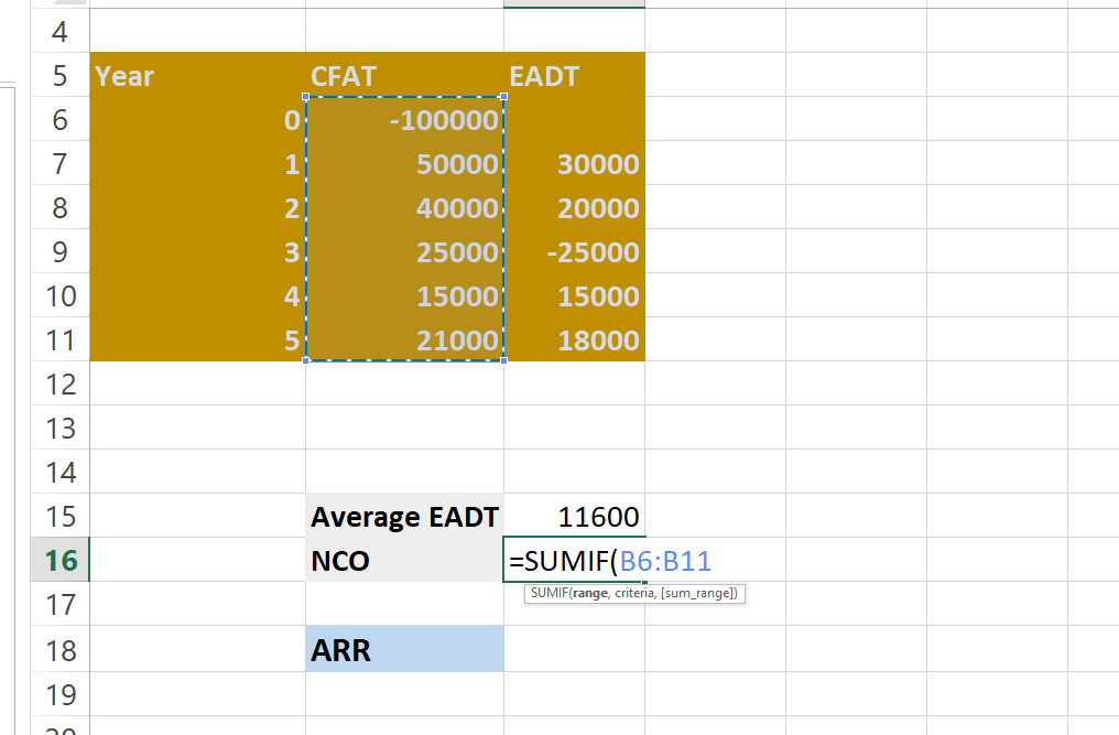
For a sum_range parameter, again select the CFAT Values. Here in our example, from B6:B11. After this, hit enter and see the NCO Result. It’s 100000 in our assumption calculation. Here we used for NCO, =SUMIF(B6:B11,”<“&0,B6:B11)
Final Calculation Using Formula
Go to ARR Cells, here we are going to calculate the ARR forecast.
Select the Average EADT, like =C15. Here are our EADT Lies in Column C15. So, you have to select the average EADT Cell. After selecting the Average EADT, input the Divide sign (/).
After the divide sign, open a bracket and select the NCO value. If the NCO is negative, then you have to enter the ABS Function.
In our case, it’s negative. So, we enter the ABS before NCO. Like this, =C15/((ABS(C16)+.
Now Select the Salvage Value, it’s in B3 in our worksheet. Like this, =C15/((ABS(C16)+B3)/
Divide the value by 2 and close the bracket. It’s =C15/((ABS(C16)+B3)/2
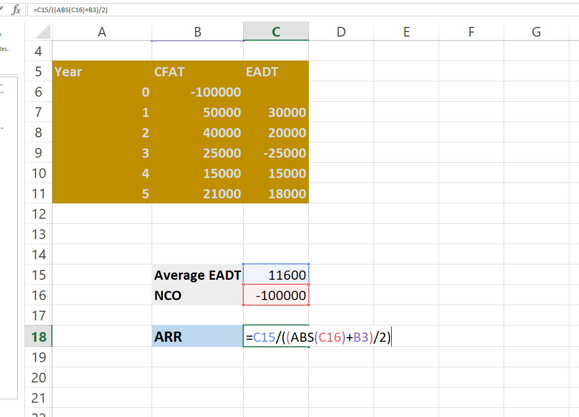
ARR = Average EADT/ (NCO + Salvage Value/2)
In Above Example =C15/((ABS(C16)+B3)/2)
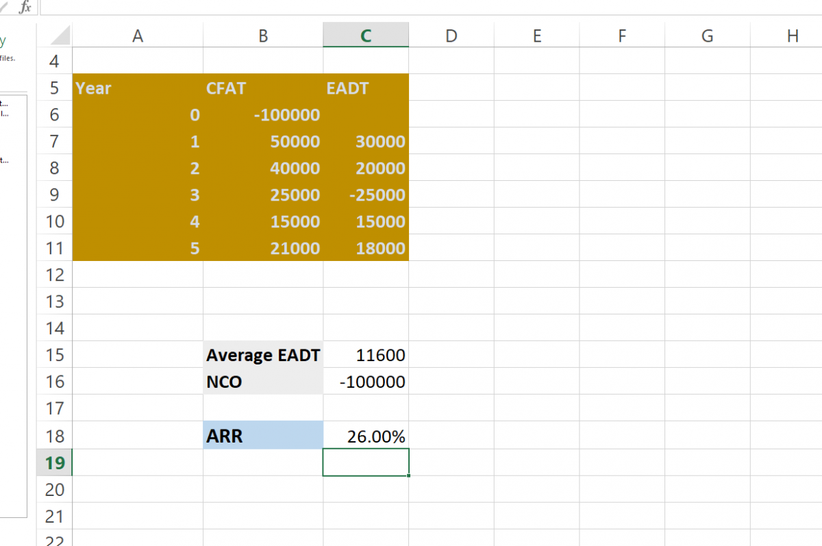
As per this calculation, we can make the decision whether to go for an investment or not.
Conclusion
That’s the end of the tutorial. Hope you have learned about ARR (Accounting Rate of Return) and how to calculate ARR in Excel and now can implement it yourself well to forecast an investment opportunity.
