This article is a detailed step-by-step guide to some cool tricks and tips using the advanced filter tool in Excel. We will also learn the fundamental uses and applications of the tool in this tutorial. So, make sure to read till the end and become a pro at the Advanced Filter tool.
Let’s get cracking!
Getting started: Advanced Filter tool in Excel
The advanced filter in Excel is located in the Data tab in the Sort & Filter group.
You can use this tool to filter duplicate entries from a data range, filter data based on criteria, or filter specific data from the range beginning with a specific alphabet, and more.
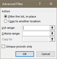
This is the advanced filter tool in Excel.
Actions: You can see two actions that can be performed:
Filter the list, in-place.
Copy to another location.
These options allow you to choose if you want the filtered results to be applied on the same range or you’d like to copy and paste the results to a different location.
It is recommended that you choose the second option as you cannot restore the previous data. Although you can Undo the changes made, you will lose the results if you select the first option.
List range: List range is the range of your list or database that you are filtering data.
Criteria range: Criteria range is selected when filtering data based on criteria.
Copy to: This option becomes available when you choose the second option. It asks you to choose a location in the workbook to paste the copied filter results.
Unique records only: This checkbox allows you to filter unique data from a range containing duplicate data.
Filtering unique data
Let’s filter unique salesperson names from a sample database below.
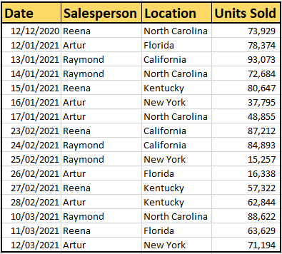
- Go to the Data tab.
- Click on Advanced under the Sort & Filter group.
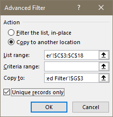
- Choose Copy to another location.
- In the List range, select the column you want to filter data from. Here, Salesperson.
- Leave the criteria range box blank.
- Check Unique records only.
- Click OK.
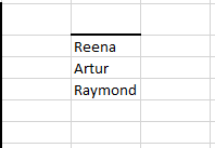
You can see the unique names filtered from the range here. If the first name or entry is repeated at the bottom of the result, delete that entry.
You can do the same for multiple columns by selecting those columns in the List range.
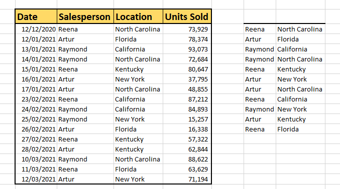
You can see the unique names with their sales location are filtered successfully.
Filtering data based on criteria
Here’s where the Criteria range comes in handy. Let’s learn to filter data based on criteria.
You can use a single criterion or multiple criteria to filter your data. Here are the steps.

- Copy the headers of the data range in the same sheet beside it.
- Type in a value for which you want to filter the entire data. For example, type Artur to filter data for Artur.

Let’s say we want to filter all the data for Artur from the range.
- Type Artur in the criteria range in the Salesperson column.
- Open the advanced filter.
- Choose Copy to another location.
- In the List range, select the entire range including headers.
- In the Criteria range, select the entire range you copied and entered a criteria value.
- Check the box if you want to filter unique records only.
- Click OK.
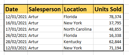
You can see that all the data for Artur has been filtered successfully.
If you wish to filter the data for multiple salespersons or a specific location or date, you can do it by entering those values in the criteria range.
Filtering data containing specific values
You can filter the data containing specific values like alphabets, numbers, or symbols.
To achieve this, you must put an asterisk (*) before or after the value. An asterisk before a value represents anything that comes before that value. An asterisk after a value represents anything that comes after that value.
Let’s say we want to filter names that start with R from the range.

- Type R* in the criteria range under the Salesperson column.
- Open the advanced filter.
- Choose Copy to another location.
- In the List range, select the entire range including the headers.
- In the Criteria range, select the criteria entire.
- Click OK.
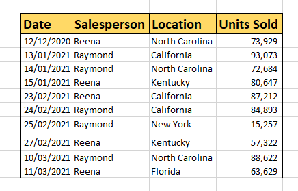
You can see that the data for Reena and Raymond have been filtered because their names start with R.
You can try entering *o in the criteria range to filter names containing O in them.
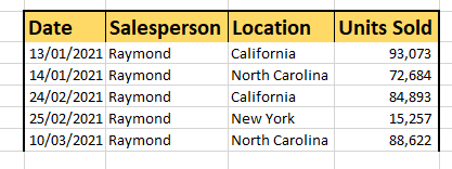
There is only Raymond with an O in his name that has been filtered.
Similarly, you can enter a criterion to filter data that contains less than or greater than a specific number.
Conclusion
This article was a detailed step-by-step guide to some cool tricks and tips using the advanced filter tool in Microsoft Excel. Stay tuned for more advanced and interesting topics like this!
