What use is it if we have a sheet full of formulae in MS Excel, but are not able to sneak a peek all at once? What’s all with the secrecy of these formulae hiding behind the textual or the numerical results which they generate? In this article, we shall get down to it and explore the ways of revealing the formula in plain sight.
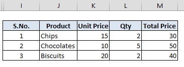
Let’s say we have a list of items purchased as shown in the below image.

Isn’t it difficult to spot those cells which are with the formulae? Oftentimes, this may cause a major setback while working in spreadsheets when we try to overwrite those contents manually or mistake the logic behind its calculation for something else, so on and so forth. So, it is always wise to know what we’ve in hand before getting on to do something with it.
Thinking of the ways to get the job done, there are actually a couple of them that could serve the purpose and each of those ways is listed down below.
- Using Formula Tab
- Using Keyboard Shortcut
1. Using Formula Tab
This one calls for the aid of only a mouse to reveal the formulae that have been used in the contents of the sheet. Make sure you are in the sheet that contains the formula that we need to have a look at.
Once that is done navigate to the Formulas tab in MS Excel & we can see a whole lot of options pertaining to different aspects of formula ready for deployment.

Now it is time for us to look for the Show Formulas command within the Formulas tab. Upon successfully locating it, click on it and all the formulae within the sheet will be rendered visible in plain sight as shown in the below image.

If you were thinking it was a multiplication formula with an asterisk in between 2 cell addresses, please tell me that I’ve caught you off guard with this!
Now click on any of the cells with the formula and it shall reveal all the cells upon which it was constructed as shown below.

In the above image, it can be noted that the Show Formulas command is highlighted inferring that it is active. So, as long as it remains active, we can only look at the formula constructed within each cell and not at its final result.
To take the worksheet back to its original state, click on the Show Formula command again and the status quo shall be restored.

2. Using Keyboard Shortcut
This is a bit quicker than the other method, saving all the hardships of searching for the required command by skimming through the list of the available tabs.
Make sure that the worksheet containing the formulae lays right before your eyes before getting starting with. Now, this is a fancy way of telling that the worksheet containing the formula should be the active worksheet.
All eyes on the keyboard now! There is a key just before the number ‘1’ on the top layer of your keyword containing a tilde (~).
Hit the CTRL key followed by that tilde key. The emphasis here is on pressing these keys one after the other since pressing them simultaneously won’t make this method work.
Once it’s done, the table turns into the format as shown in the below image.

To bring it back to its previous state, repeat pressing the CTRL key and the tilde (~) key. The table returns to its previous state like a charm!

Conclusion:
So, there it is, two different methods to display the formula used within an active worksheet for your usage. To know more about similar shortcuts and tricks on using MS Excel, do watch out QuickExcel. Adios!
