In this tutorial, you’ll learn how to perform Linear Regression in Excel. Linear regression is an approach to linear modeling the relationship between a dependent and an independent variable. Simple linear regression uses an independent variable to predict the outcome of the dependent variable.
The equation for linear regression is given by: y = a + bx, where x is the independent variable, y is the dependent variable and the coefficients are given by:
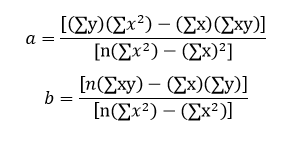
Our aim is to find coefficients a which is the intercept and b which is the slope to obtain the equation of the straight line which best fits our data by the least square method. There are two ways in Excel in which we can find the linear regression line which is discussed below for the following data set:
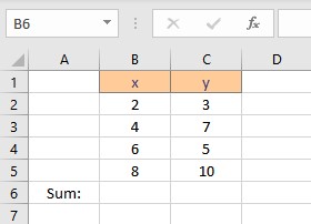
Calculate Linear Regression in Excel Using Its Formula
First, we need to calculate the parameters in the formula for coefficients a and b. The parameters are Σx, Σy, Σxy and Σx2 . To calculate Σx follow these steps:
- Select the cell where you want to calculate and display the summation of x.
- Type =SUM(, select the cells containing the numbers and complete the formula with ).
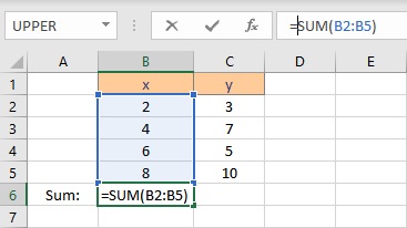
- Press the Enter key to display the result.
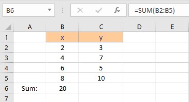
To calculate Σy follow these steps:
- Select the cell where you want to calculate and display the summation of y.
- Type =SUM(, select the cells containing the numbers and complete the formula with ).
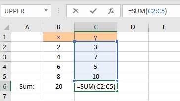
- Press the Enter key to display the result.
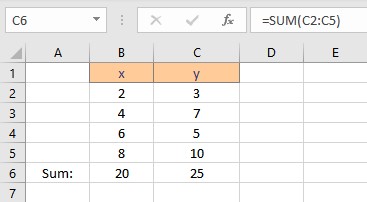
To calculate Σxy follow these steps:
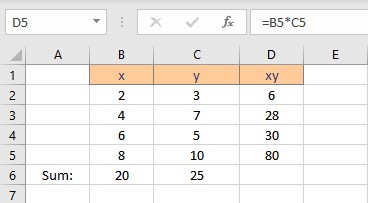
- Select the cell where you want to calculate and display the product of a pair of x and y values.
- Type =B2*C2, as the first x and y values are in cells B2 and C2 respectively.
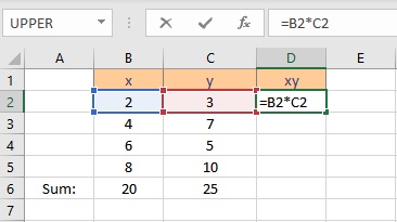
- Press the Enter key to display the result.
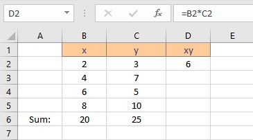
- Copy the formula for the calculation of product xy for the entire list by dragging down the fill handle.
- Select the cell where you want to calculate and display the summation of xy.
- Type =SUM(, select the cells containing the numbers and complete the formula with ).
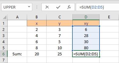
- Press the Enter key to display the result.
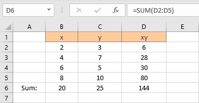
To calculate Σx2 follow these steps:
- Select the cell where you want to calculate and display the square of the first x value.
- Type =B2^2, as the first x value, is in cell B2. The caret operator raises the number to the power written next to it.
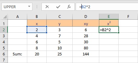
- Press the Enter key to display the result.
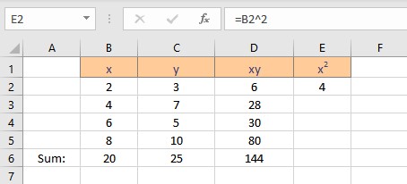
- Copy the formula for the calculation of squares of x for the entire list by dragging down the fill handle.
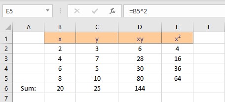
- Select the cell where you want to calculate and display the summation of x2.
- Type =SUM(, select the cells containing the numbers and complete the formula with ).
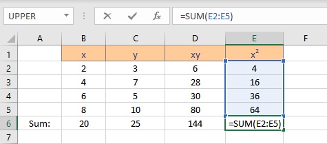
- Press the Enter key to display the result.
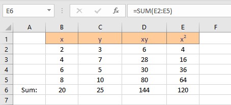
We now have the parameters essential for the calculation of coefficients intercept a and slope b. Follow the steps to calculate the intercept a:
- Select the cell where you want to display the value of the intercept.
- Type =(C6*E6-B6*D6)/(4*E6-B6^2), where C6 contains the value of Σy, E6 contains the value of Σx2, B6 contains the value of Σx, D6 contains the value of Σxy and 4 is the number of data points in the data set.
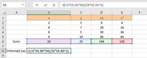
- Press the Enter key to display the result.
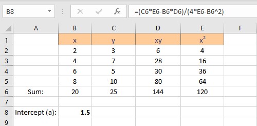
Follow the steps to calculate the slope b:
- Select the cell where you want to display the value of the slope.
- Type =(4*D6-B6*C6)/(4*E6-B6^2), where C6 contains the value of Σy, E6 contains the value of Σx2, B6 contains the value of Σx, D6 contains the value of Σxy and 4 is the number of data points in the data set.
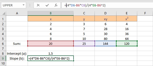
- Press the Enter key to display the result.
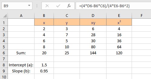
We have the values for the slope and intercept, the equation for the linear regression can be written as y = 1.5 + 0.95x. This equation can now be used to predict values of y for different values of x.
Linear Regression in Excel Using Data Analysis
To use the Data Analysis feature, you need to enable Analysis Toolpak in Excel. Follow these steps to manually enable the feature:
- Click on the File option present at the top left corner of the Excel window.
- From the menu that appears, click on Options to launch the Excel Options dialog box.
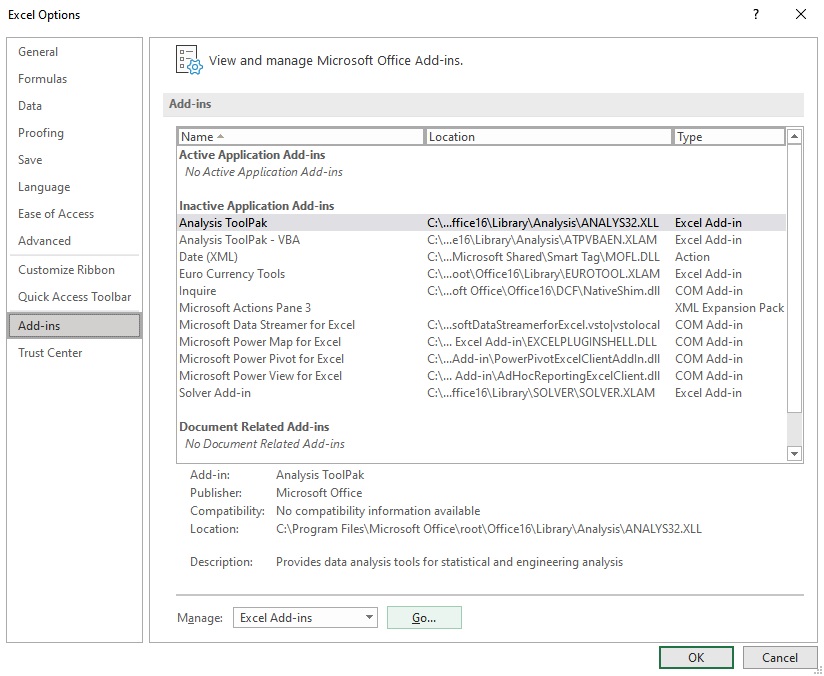
- Select the Add-ins option at the left side of the Excel Options dialog box.
- Select Excel Add-ins in the Manage box, and click Go.
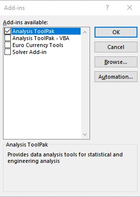
- In the Add-ins dialog box, check the Analysis Toolpak checkbox, and then click OK.
- The Data Analysis option now appears in the Analysis group on the Data tab.

Follow these steps to perform linear regression using Data Analysis:
- Click on Data Analysis present in the Analysis group on the Data tab.
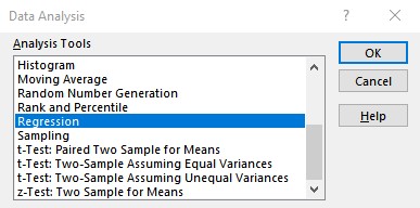
- From the Data Analysis dialog box that appears, select Regression under the Analysis Tools and click on OK.
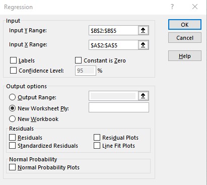
- Enter the cell ranges containing y values in the Input Y Range: text box and x values in the Input X Range: text box in the Regression dialog box and click OK.
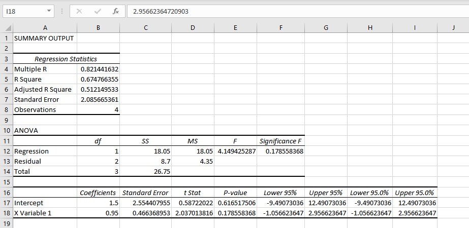
- The results are displayed in a new worksheet. You can copy the intercept and slope coefficients to obtain an equation for the linear regression: y = 1.5 + 0.95x.
Conclusion
In this tutorial, we learned how to perform linear regression both using the formulas and Excel Add-ins.
