There would be times at which one needs to verify whether the data available in a particular tabulation is also present in a different tabulation which sometimes might be in a different sheet. While one can switch between the sheets and verify each item one after the other, it defeats the sole purpose of using MS Excel! What difference is this to verifying manually between the information recorded in two notebooks?
In this article, we would be covering a technique which will get the job done without much hassle and a formula will be put into use to make this happen – the VLOOKUP!
VLOOKUP – What it is?
Following is the syntax of Vlookup which contains all the basic constructs needed for its proper functioning,
=VLOOKUP(lookup_value, table_array, col_index_num, [range lookup])
where,
- lookup_value – the item which is to be searched elsewhere (source)
- table_array – the destination table within which the item is to be searched
- col_index_num – the column position from the start of the destination table whose value is to be returned
- [range lookup] – an optional element set to FALSE (0) by default to return the value that exactly matches the search item. In case the requirement is to get an approximate match, this can be changed to TRUE (1).
With all these elements filled in, this formula shall return a value against a search item after thoroughly screening the selected destination table.
Comparing 2 Columns from Different Sheets in Excel
Let us consider the following data which has a list of items.
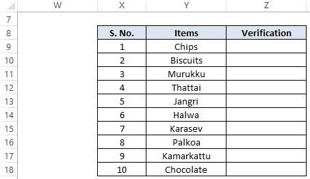
There is an empty column at the end of the above tabulation titled ‘Verification’. So, what we are going to demonstrate is to verify whether each item listed in this tabulation is present in another list of data given in another sheet.
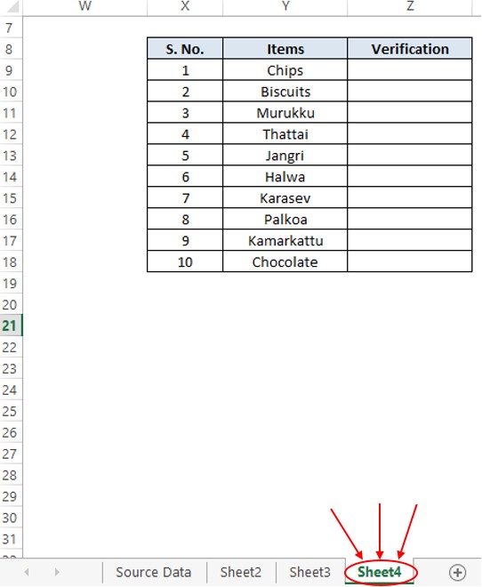
From the above image, it is evident that the source list whose data is to be verified is in Sheet 4. Here’s another list in Sheet 3 which contains the sales data of the different items listed in Sheet 4.
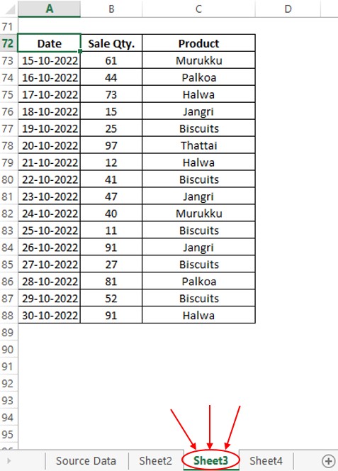
Our objective here is to construct a Vlookup formula in the Sheet 3 list to compare it with the list in Sheet 4. Let us get started by double-clicking on Z9 in Sheet 4 to include an equals sign (=) followed by typing Vlookup and an open round parenthesis as shown below.
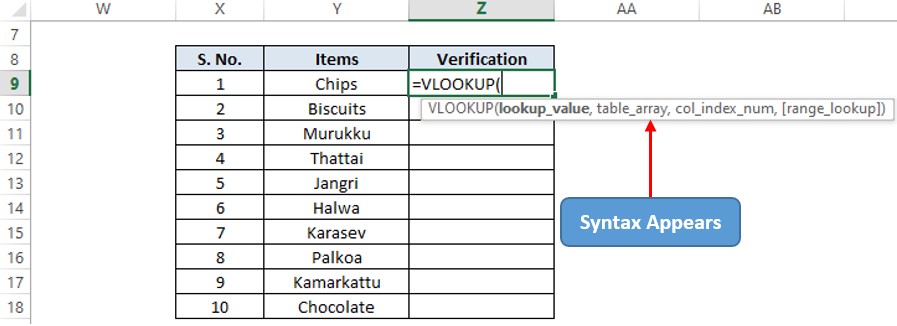
The lookup value will be those in column Y which in this case would be ‘Chips’. So click on the cell Y2 and include a comma.
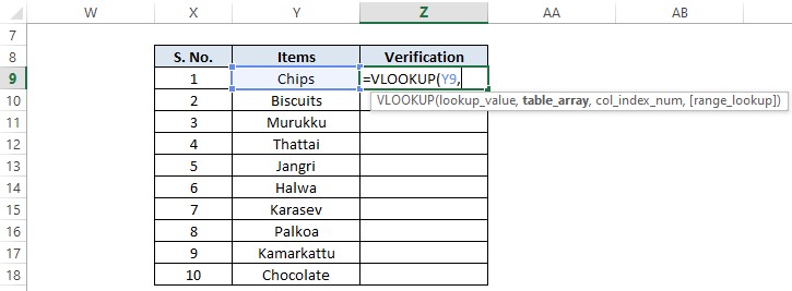
Now it is time to select the Table array & we shall get into sheet 3 to select the column with the items listed.
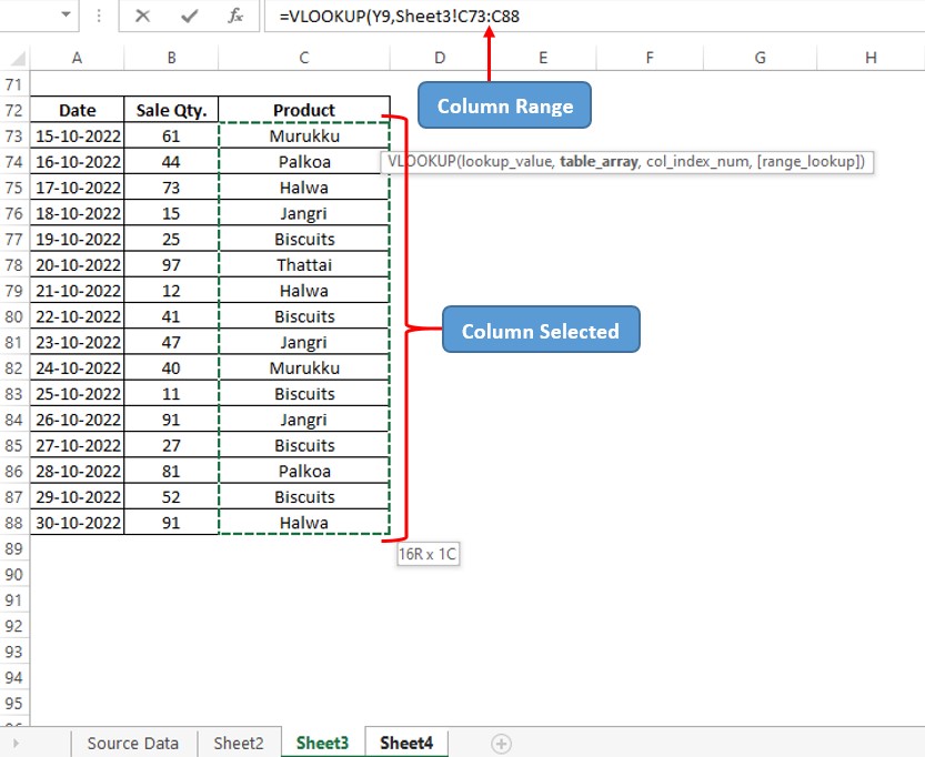
Now, remember to make this column selection an absolute reference since the selected column will change when this formula is copied & pasted to other cells due to the inherent auto-adjusting feature of MS Excel.
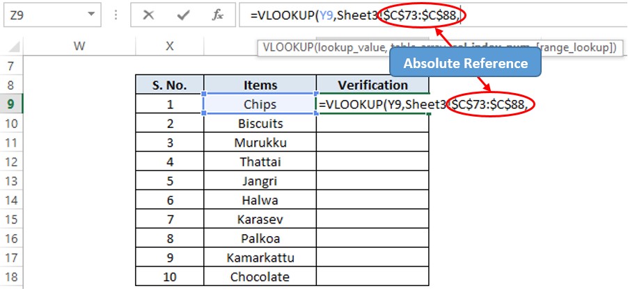
Since we have selected only one column in Sheet 3, the column index number shall be ‘1’. Type ‘1’ after the comma following the table array & include another comma after typing it.
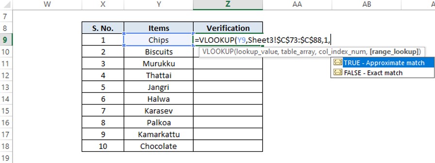
We would only be needing exact matches for these item names, so we shall choose FALSE. We can type ‘0’ too rather than typing FALSE in the formula & then close the round parenthesis.
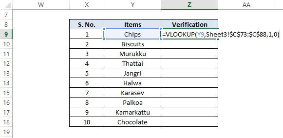
Hit ENTER & if ‘Chips’ is available in the list of items in Sheet 3, the result shall be ‘Chips’ else a #N/A (Not Available) error shall appear.
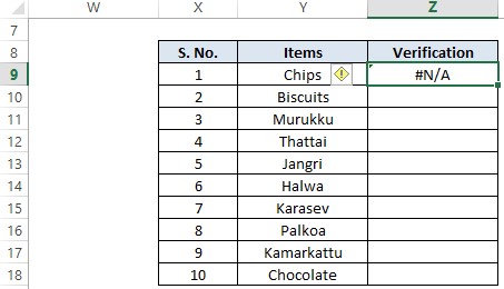
Copy this formula & paste it across all the cells below to know the results of whether they are available in the list in Sheet 3.
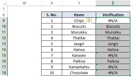
It seems that S. No. 1, 7, 9 & 10 aren’t available in the Sheet 3 list.
Conclusion
Now we have reached the end of this article, hope it has provided you with sufficient clarity on comparing two columns using Vlookup. Have a look at this article, if you would like to know about using $ in formulae of MS Excel. For more cool tricks on using MS Excel, please do look into our space QuickExcel. Until then, Ciao!
