Rather than sitting on its laurels, Microsoft has been constantly updating its Office Package with new features to make life easier for its users. As a part of this package, MS Excel also gets its own share of new features in every update & one such update is the ‘Dynamic Arrays’.
Before this feature was introduced, one needs to construct a formula for handling multiple values across a column & use flower brackets ‘{ }’ for MS Excel to read that it ain’t a regular formula, followed by pressing CTRL+ENTER to get the results. But with the homecoming of the ‘Dynamic Arrays’ feature, this all ends.
Also read: How to Fix #N/A Error in MS Excel?
Let us consider the following data for instance, for which we need to find the list of unique values (i.e) stripping the list of the repetitions.
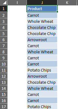
Without ‘Dynamic Array’ we either need to copy this list to a new column & use ‘Remove Duplicates’ to find the list of unique values or to write a lengthy, complicated array formula to get the job done. But now, one is saved from the misery of going through these by making use of UNIQUE!
=UNIQUE (array, [by col], [exactly once])
Given above is the syntax for this ‘Dynamic Array’ formula where,
- array – the range of cells which is to be analysed
- [by_col] – an optional construct in which TRUE is to be given for returning unique values across columns & FALSE is to be given for returning unique values across rows
- [exactly_once] – an optional construct in which TRUE is to be given for returning items that appear exactly once & FALSE is to be given for returning every distinct item
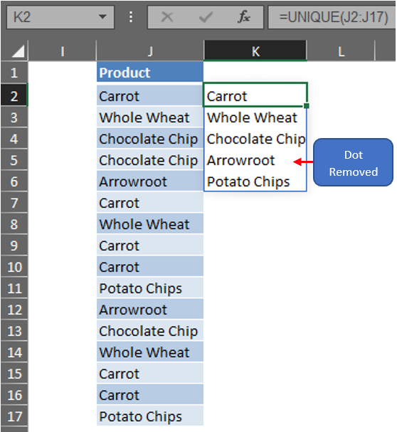
TRUE is the default selection for the optional constructs given above. Let us now use this formula for extracting the unique values from the list given earlier.
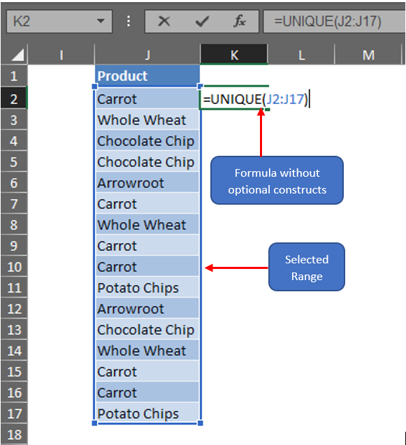
One could observe that the optional constructs are omitted from the above formula & only the range of cells to be analysed is selected. Hit ENTER & you are in for a surprise!
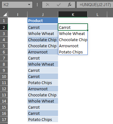
The formula hasn’t been pasted across the cells – NO! Once ENTER is hit, the formula has itself adjusted to fill all the unique values across the column in which it has been constructed. Such is the power of the ‘Dynamic Array’. “Enough praises for this new feature & where is the #SPILL error?” you ask. We are heading there!
The Advent of #SPILL Error:
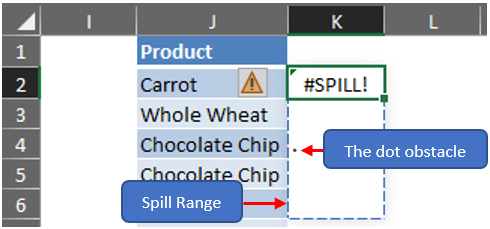
Have a look at the image below.
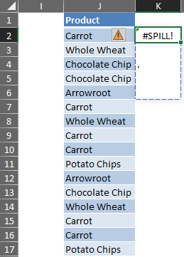
Something has stopped our UNIQUE formula from spilling the results across the column (Yep, you’ve guessed it right! Since it prevents spilling of the formula, thusly the name #SPILL error). Upon closer observation, it can be seen that there’s a dot ‘.’, a tiny dot within the range in which the results are to be spilt.
Remove this dot ‘.’ & the formula will work like a charm!
#SPILL Error in Table:
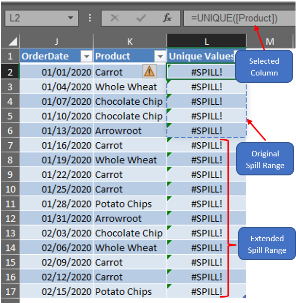
Things slide from bad to worse when ‘Dynamic Arrays’ are deployed in Tables. The inherent feature of the table to apply a formula typed in any cell of a column defeats the very purpose of using this formula. The following error comes up when the entire range of column K is selected within the UNIQUE formula.
The error can be removed using the implicit intersection operator ‘@’ as shown below. What this does is rather than using the entire array, it makes the formula in a particular cell only use the corresponding single cell value.
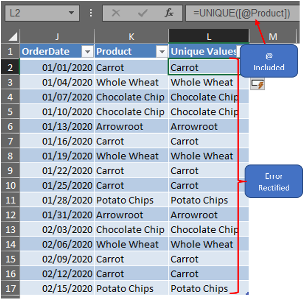
But these results don’t provide any meaningful inference. Thusly, dynamic array formulae are better not to be used within the tables.
Summary
Have a look at this article which elaborates further on the usage of ‘@’ within the formulae. There are numerous other articles in QuickExcel that can help you to learn the tricks & nuances of using MS Excel. Cheers!
